How To Build a Neural Network From Scratch in Python
Neural networks are one of the most interesting and thriving topics in today’s computer science research landscape. Many of the discoveries made in recent years will impact, in various degrees, the way we work and the way we make art. Technologies such as Generative Adversial Networks(GAN), Autoregressive Models(AR) and Diffusion Probabilistic Models are a clear example of the capabilities of deep learning applied to the real world.
Over the years, many libraries and frameworks, such as Tensorflow, have made the task of training and using a neural network as simple as possible, even for those who do not want to fully dive into the math part of machine learning. But while this is a great way to build AI-powered apps in no time, it is not optimal to treat a neural network as a mysterious device, where you do not understand what is going on and how they actually manage to produce a certain result. In this guide we will try to understand the theory and the math behind a simple multilayer perceptron. We will then try to build one from scratch by ourselves, and finally we will use it to make some predictions.
How Does a Compute Learn From Data?
To understand how a computer learns from data, think about how human brains do this kind of activity. For example, suppose you have to teach your newborn child how to recognize a dog. What is the first, most natural thing to do? You show them a picture of a dog, of course! Then, when they will come across a dog on the street, their brain will be able to recognize the dog. But what if the child misrecognize another animal, let us say a cat, for a dog? In that case you correct them by pointing out which animal is actually the dog. In that way, their brain will correct their knowledge on how to recognize a dog.
This is pretty much how a computer learns from data: we train a mathematical model by providing examples of solutions of the problem we are trying to solve, and at each iteration we update the model until we achieve a low error rate. Once we have done that, the model is ready to make predictions.
Let us try to make an example: suppose to have a function like the following:
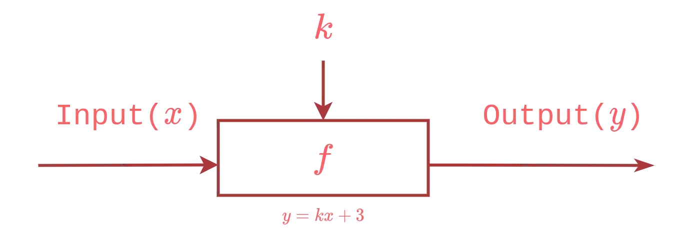
where the output($y$) is determined by the formula $y = kx + 3$ and $k$ is the model of the function, i.e. the parameter to be trained. Let us start the training process by letting $x = 5$ and $y = 21$. Let also choose a random value for the function parameter, for example $k = 1$.
The first step of the learning algorithm is the following: 1. $$ k = 1 $$
$$ y = 1 \cdot 5 + 3 = 8 \neq 21 $$
$$ E = | 21 - 8 | = 13 $$
As you can see the error(the difference between the expected value and the actual value) is too high, so we iteratively repeat this process until it is near zero. For the next iteration, we will set the parameter $k = 6$ $$ k = 6 $$
$$ y = 6 \cdot 5 + 3 = 33 \neq 21 $$
$$ E = | 21 - 33 | = |-12| = 12 $$
That’s too much! Let’s trim it again: $$ k = 4 $$
$$ y = 4 \cdot 5 + 3 = 23 \neq 21 $$
$$ E = | 21 - 23 | = |-2| = 2 $$
$$ k = 3.5 $$
$$ y = 3.5 \cdot 5 + 3 = 20.5 \neq 21 $$
$$ E = | 21 - 20.5 | = .5 $$
$$ k = 3.6 $$
$$ y = 3.6 \cdot 5 + 3 = 21 $$
$$ E = | 21 - 21 | = 0 $$
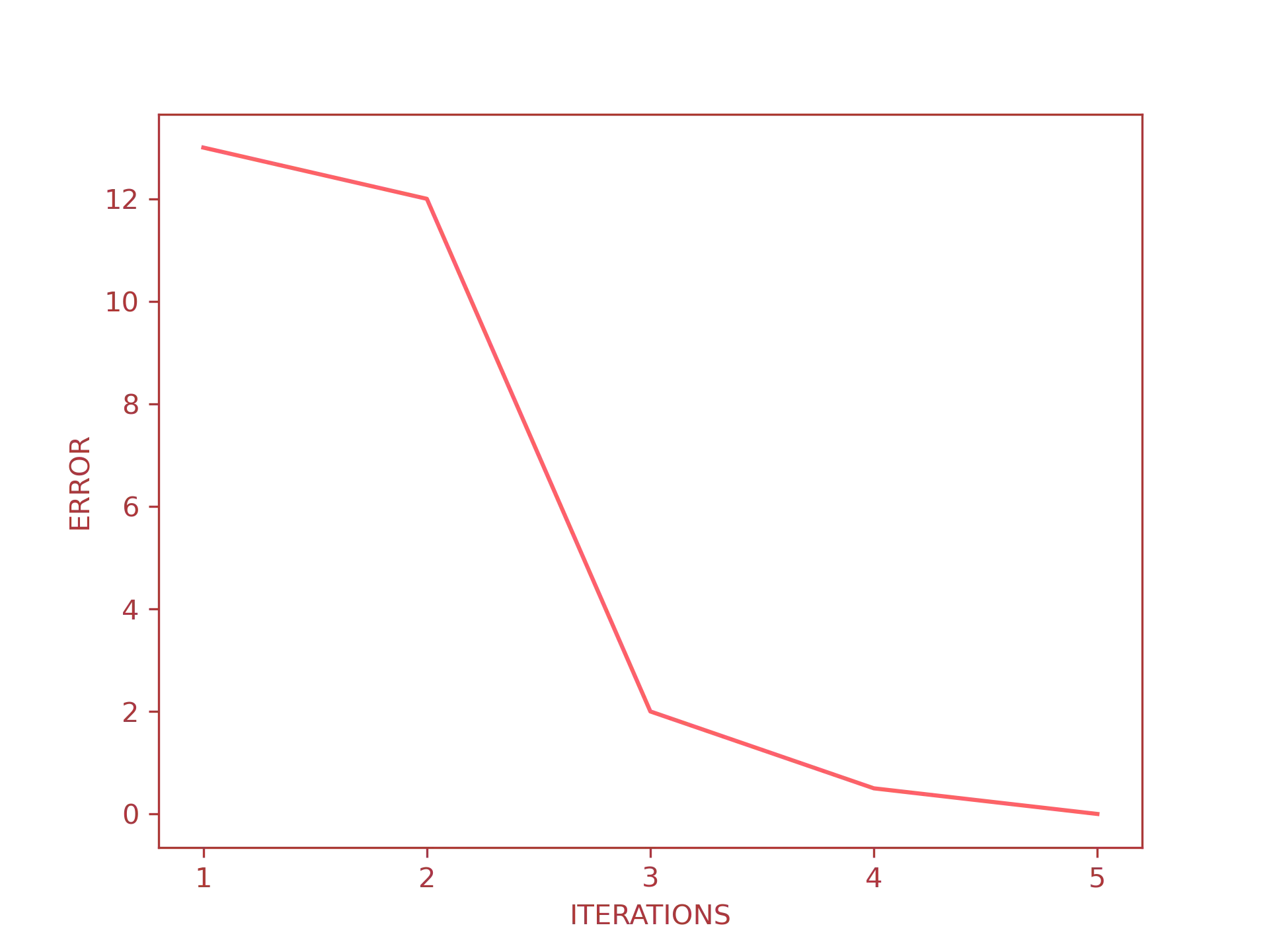
We did it! The target value is $k = 3.6$, meaning that the function is now trained and ready to make predictions. We can also try to plot the iterations vs the error to actually see the error descent at each iteration:
This is what machine learning is all about: the mathematical model gets updated at each iteration by computing the error; once the error is lowered at a tolerable level, it is ready to make predictions. Quite easy, at least from an abstract point of view, but in order to write a neural network all by ourselves, we need to understand how they work under the hood.
Neurons
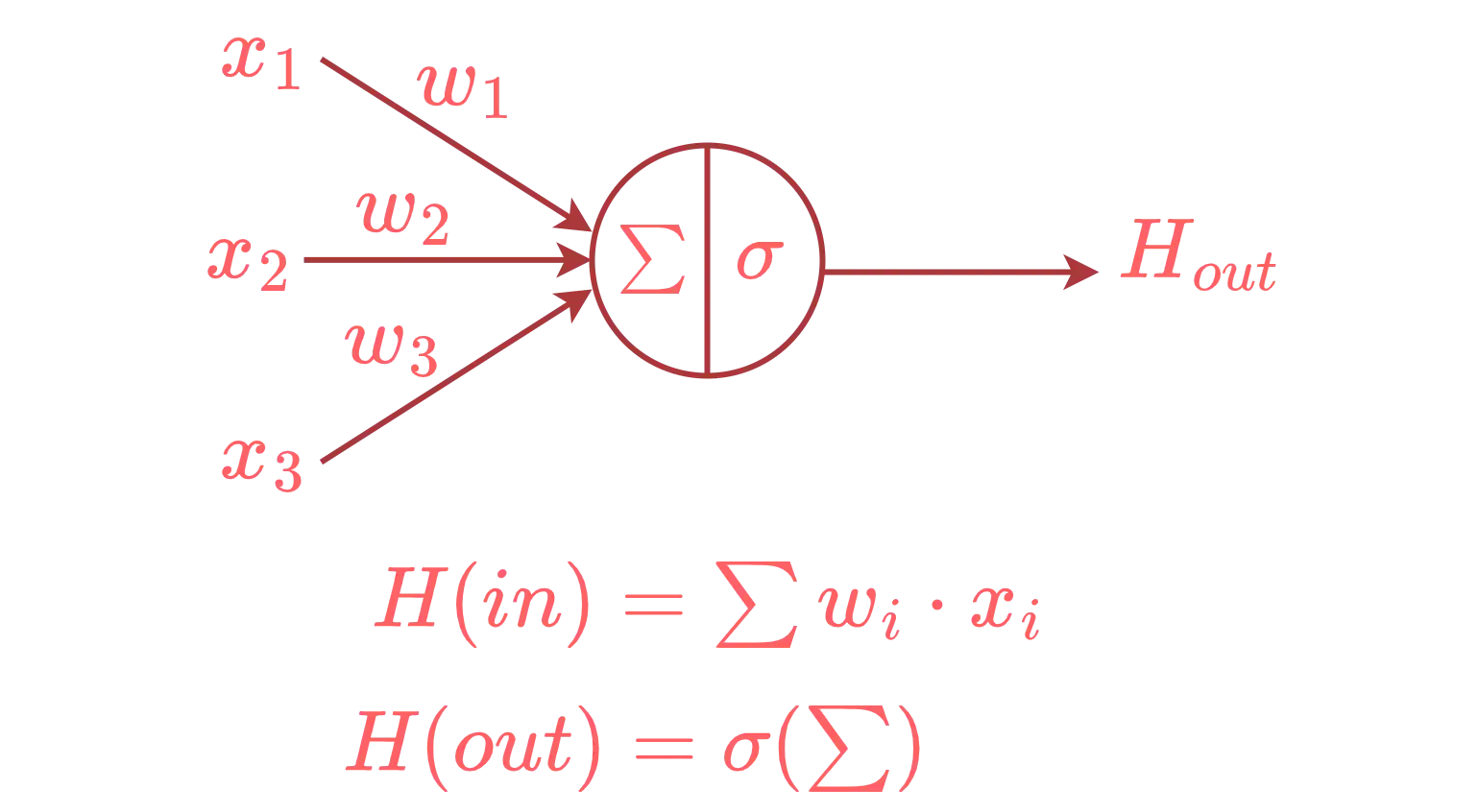
The core element of every (artificial) neural network is the neuron. In a human brain, a neuron is a nerve cell that receives some inputs, process them and transmits the output through electrical signals to other neurons. The connection between each neuron is called a synapse.
When the input signals are strong enough, the neuron triggers a new signal that will be sent to other neurons. This is exactly how artificial neural networks works: each neuron receives some inputs, and when they are “strong” enough, a new signal will be propagated to the next neuron of the network.
The only differences is that an artificial neuron is just a mathematical function, the “strength” of a signal is called the weight and the output signal is determined by an activation function. Graphically this is how a single artificial neuron looks like:
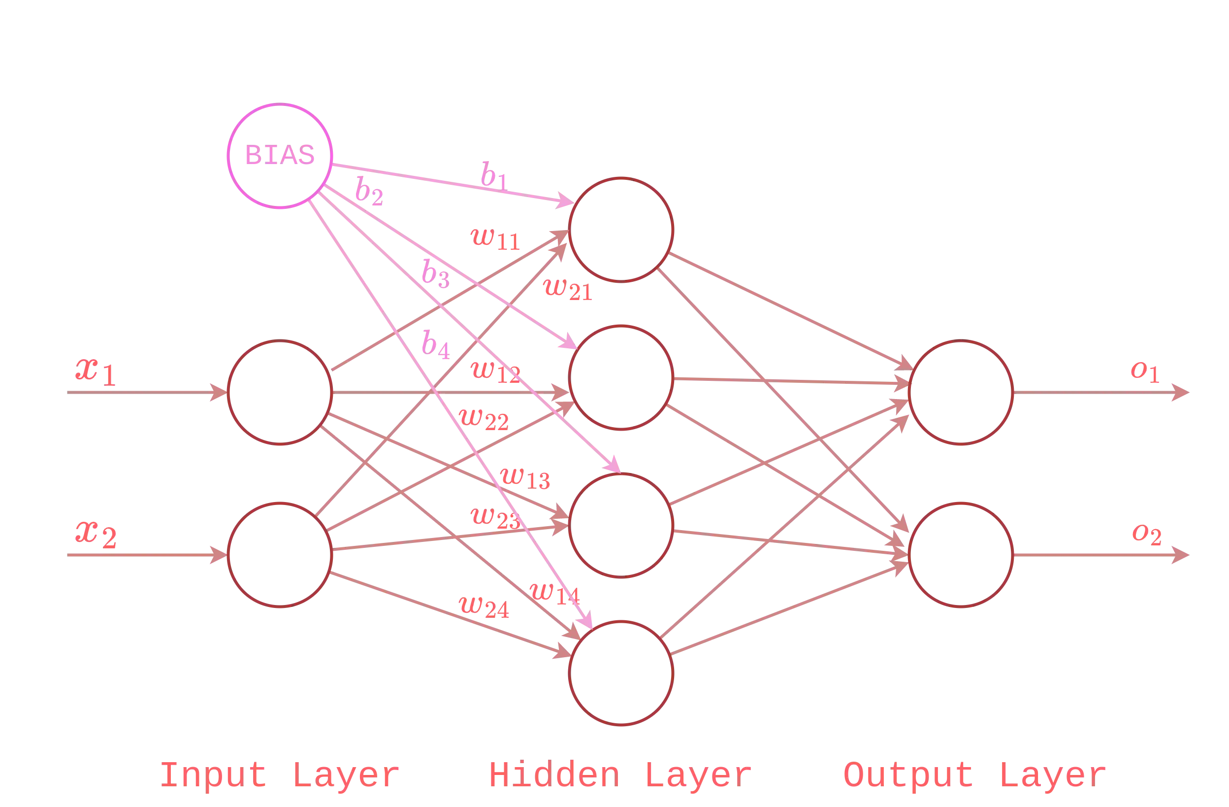
and this is how a fully connected network of neurons(i.e., a neural network) looks like:
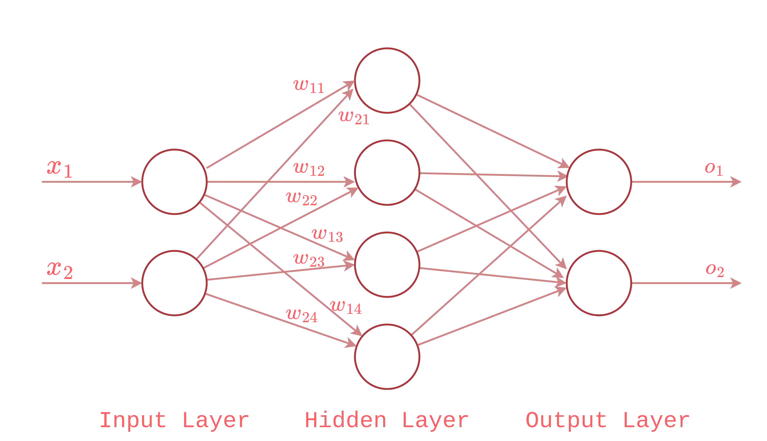
where the input layer - formed by two neurons - sends its output to the hidden layer which finally sends its output to the output layer. As you can see, each connection from the input layer to the hidden layer has a weight, this is one of the configurable parameter that allows us to train the neural network.
In the next section will learn the steps involved in the learning process but first, let us find out an appropriate algebraical structure to efficiently compute the output of the network. As you may have noticed, calculating the result of $\sum w_i \cdot x_i$ of any neural network(even the small example above) is quite inconvenient. The preferred way to do this, is to represent the inputs and the weights as matrices and then to use linear algebra rules to compute their dot product, i.e.:
$$ \begin{bmatrix} x_1 \ x_2 \end{bmatrix} \cdot \begin{bmatrix} w_{1,1} & w_{2,1} \\ w_{1,2} & w_{2,2} \\ w_{1,3} & w_{2,3} \\ w_{1,4} & w_{2,4} \end{bmatrix} $$
$$ = \begin{bmatrix} (x_1 \cdot w_{1,1}) + (x_2 \cdot w_{2,1}) \\ (x_1 \cdot w_{1,2}) + (x_2 \cdot w_{2,2}) \\ (x_1 \cdot w_{1,3}) + (x_2 \cdot w_{2,3}) \\ (x_1 \cdot w_{1,4}) + (x_2 \cdot w_{2,4}) \end{bmatrix} $$
Learning Process
Now that we have an idea of how neural networks are structured, we can move forward to the actual learning process. The steps needed to train a neural network can be briefly described using the following algorithm:
- Randomly initialize the weights of each neuron;
- Compute the dot product and then pass it to the activation function(forward pass);
- Compute the error using the mean squared error formula;
- Feed back the error to update the weights(backward pass);
- Update the weights;
- If the error is not within an acceptable range, repeat steps from 2 through 6.
We can divide this algorithm in two branches: the forward pass and the backward pass. Let us start with the first one.
Forward Propagation
Once we have randomly initialized the weights of each neuron, we are ready to compute the forward step, which consists in the following mathematical operations:
- dot product $\sum w_i \cdot x_i$, where $w$ is the weights vector and $x$ is the input vector.
- activation function $\sigma(\sum)$, where $\sigma$ is an activation function.
We talked about activation functions when we first introduced neurons from the point of view of human brains. Let us quickly recap what an activation function is:
An activation function is a mathematical function that determines whether the weighted sum of a neuron should fire an output signal or not.
To understand why we need an activation function, let us go back to the notion of neurons. From our perspective, a neuron is nothing but a mathematical function with one or more input and at least one output. Neuron inputs can be any kind of value in the range of $(-\infty,+\infty)$, so in order to decide when the input is “enough” to fire the output signal, we need a discriminator, which turns out to be our activation function.
There are many types of activation functions, the most common are the following:
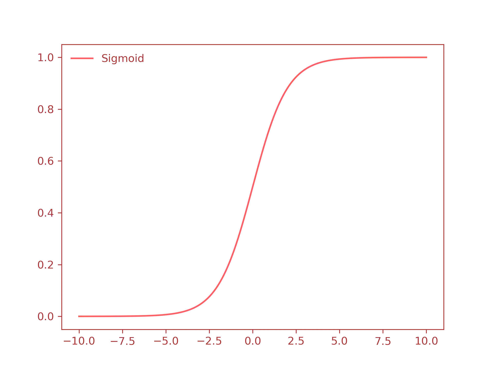
- Sigmoid: a special case of logistic function, defined as:
$$ f(x) = \dfrac{1}{1 + e^{-x}} $$
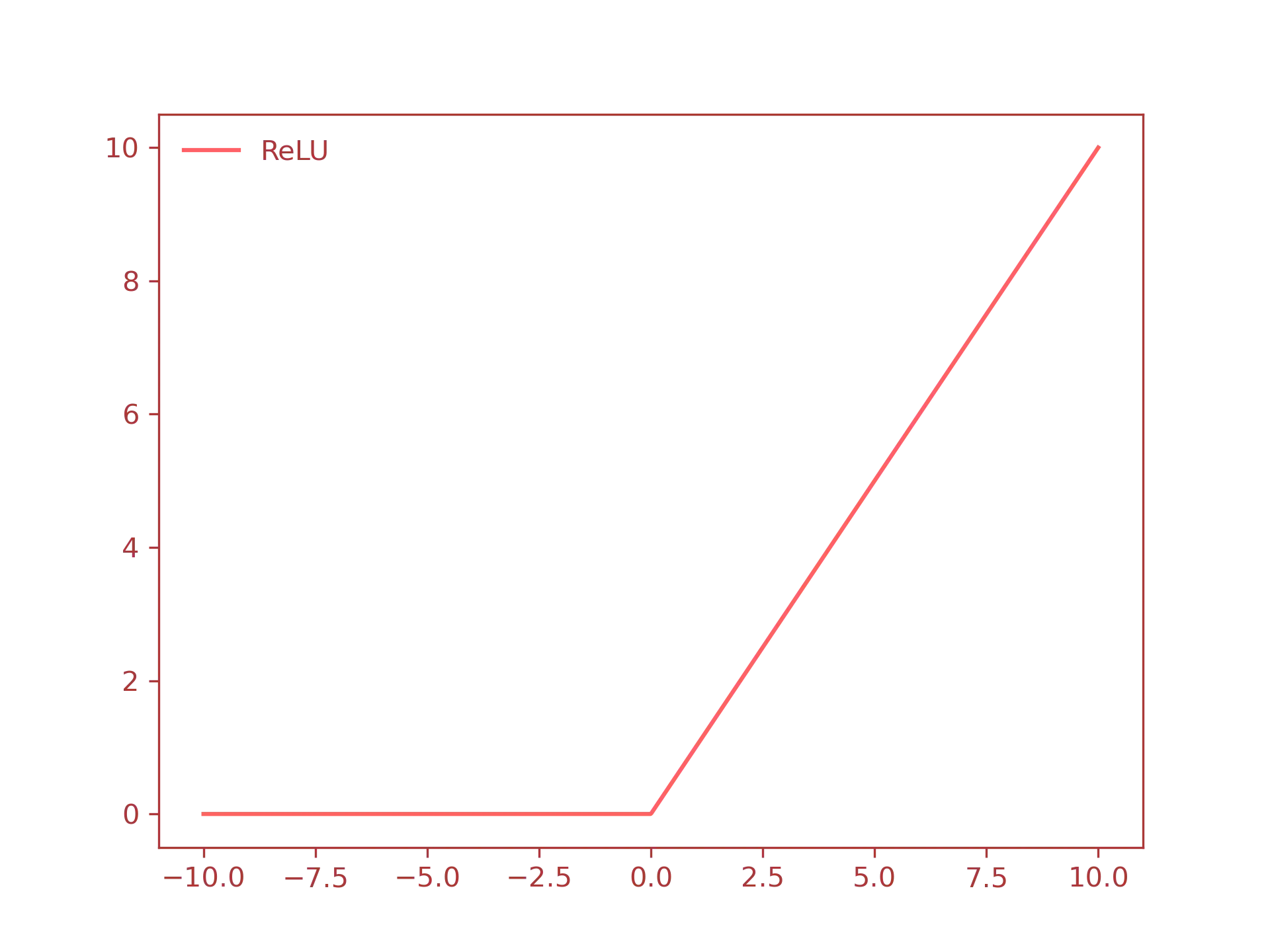
ReLU: the Rectified Linear Unit activation function, defined as: $$ f(x) = \max(0, x) = \begin{cases} x & \text{if} \ x > 0\ 0 & \text{otherwise} \end{cases} $$
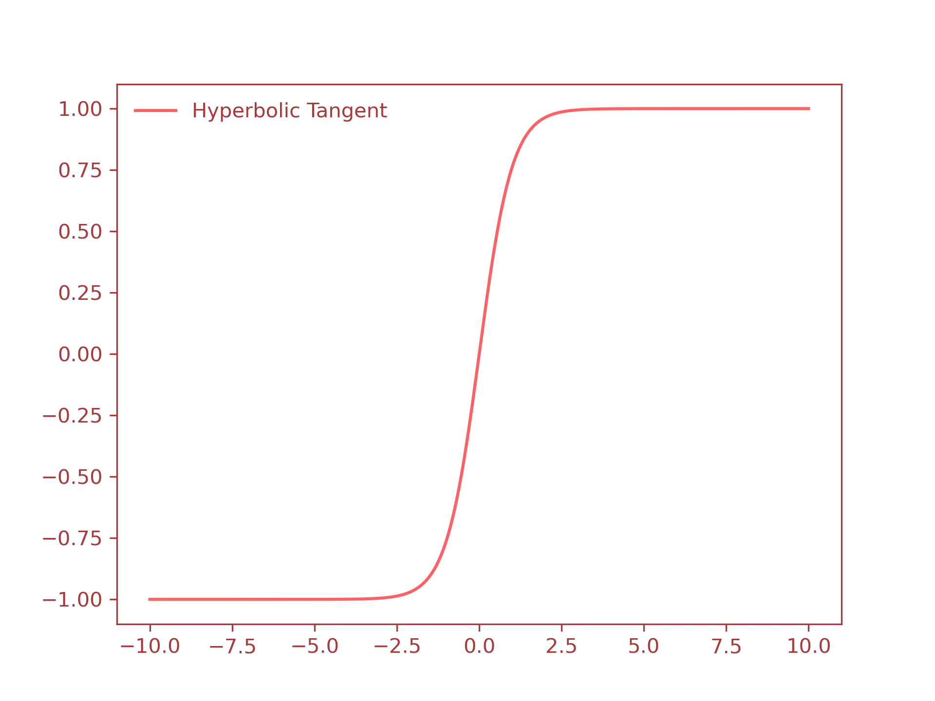
Tanh: hyperbolic tangent, defined as: $$ f(x) = \dfrac{e^x - e^{-x}}{e^x + e^{-x}} $$
Below there’s the plot of each function:
- Sigmoid function:
- ReLU function:
- Tanh function:
For the rest of this guide we will use only the sigmoid function, but keep in mind that in real world applications you will use different activation functions, such as the ReLU function.
In conclusion, the last step of the forward pass is to compute the sigmoid function of the previous result. After that, we need to compare the expected output (i.e., the result of the activation function) with the the predicted output and then feedback this difference(i.e., the error) to update the weights of each neuron. This step is called backpropagation, and it is the topic of the next section.
Backward Propagation
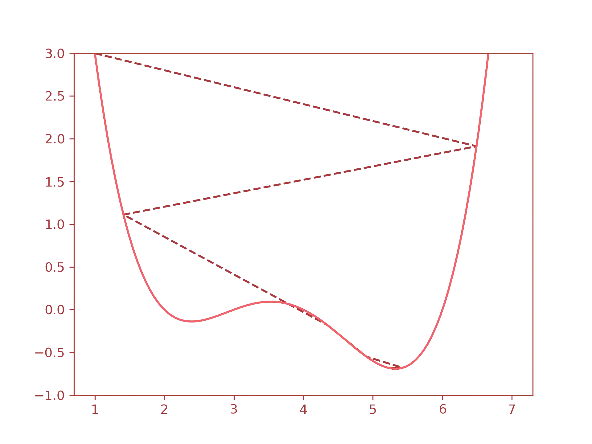
The backpropagation pass uses the gradient descent algorithm to update the weights
of the hidden and output layers. The gradient descent finds the minimum of the error
gradient; i.e., the weight vector analogous to where the error is minimal.
Visually, this is what happens when the gradient descent to the
minimum:
The first step of backpropagation is to compute the loss of the activation function using the mean squared error(MSE) defined as follows:
$$ MSE := \dfrac{1}{n} \sum_{n=1}^n (y_i - \hat{y}_i)^2 $$
In our case, we defined the error as the difference between the expected output($t$) and the predicted output($y$), i.e., the result of the activation function from the forward pass. In other words: $$ Error = (t - y) $$
The problem with this difference is that it may result in a negative error. In the first part of this tutorial, when we implemented a “predictor”, we solved this problem by taking the absolute value of the error, in this case, instead, we will use the squared error: $$ Error = (t - y)^2 $$
Finally, we divide this error by two to simplify the computations involved in the next step: $$ Error = \dfrac{1}{2} \cdot (t -y )^2 $$
In order to update the weight of each node/neuron, we need to “extract” the single errors from the total error. To do that, we will take the partial derivative of the error respecting to each weight: $$ \dfrac{\partial Error}{\partial w} $$
Let us start with the output layer(chain rule applied here): $$ \Delta_{w_o} = \dfrac{\partial Error}{\partial y_o} \cdot \dfrac{\partial y_o}{\partial a_o} \cdot \dfrac{\partial a_o}{\partial w_o} $$
which becomes:
$$ \Delta_{w_o} = (t - y_o) \cdot y_o \cdot (1 - y_o) \cdot x_o $$
where $x_o$ is the output of the hidden layer, which can further expanded with the usage of the chain rule: $$ \Delta_{w_h} = \dfrac{\partial Error}{\partial y_o} \cdot \dfrac{\partial y_o}{\partial a_o} \cdot \dfrac{\partial a_o}{\partial x_o} \cdot \dfrac{\partial x_o}{\partial a_h} \cdot \dfrac{\partial a_h}{\partial w_h} $$
which becomes:
$$ = (t - y_o) \cdot y_o \cdot (1 - y_o) \cdot w_o \cdot x_o \cdot (1 - x_o) \cdot x_h $$
where $x_o$ is the input of the hidden layer and $x_h$ is the input of the hidden layer. The partial derivative $\dfrac{\partial x_o}{\partial a_h}$ is the derivative of the sigmoid function:
$$ \sigma(x) = \dfrac{1}{1 + e^{-x}} $$
in fact:
$$ \sigma’(x) = \dfrac{d}{dx} \sigma(x) = \sigma(x)(1 - \sigma(x)) $$
Now that we have took aside each error from the total error according to the singular weights, we can use them to update the weights. To do that, we simply compute the dot product of the output/hidden layer output and the error of the output/hidden layer, respectively, i.e.:
$$ \begin{bmatrix} w_{1,1} & w_{2,1} \\ w_{1,2} & w_{2,2} \\ w_{1,3} & w_{2,3} \\ w_{1,4} & w_{2,4} \end{bmatrix} \cdot \begin{bmatrix} e_1 \\ e_2 \end{bmatrix} $$
$$ = \begin{bmatrix} (w_{1,1} \cdot e_1) + (w_{2,1} \cdot e_2) \\ (w_{1,2} \cdot e_1) + (w_{2,2} \cdot e_2) \\ (w_{1,3} \cdot e_1) + (w_{2,3} \cdot e_2) \\ (w_{1,4} \cdot e_1) + (w_{2,4} \cdot e_2) \end{bmatrix} $$
We repeat this process until the error rate is minimum. The last thing left to do before starting to write some code, we have one last thing to understand: the bias
Bias
The last component of our neural network is the bias. A bias is a configurable parameter that is added to the activation function during the forward pass. This value is used to shift the slope of the activation function to the right or to the left. Let us understand why we need it.
By default the slope of our activation function(in this case the Sigmoid) changes according to the weight of the input. For example, this is how the weights $2.0, \ 1.0, \ 0.5$ affect the steepness of the curve:
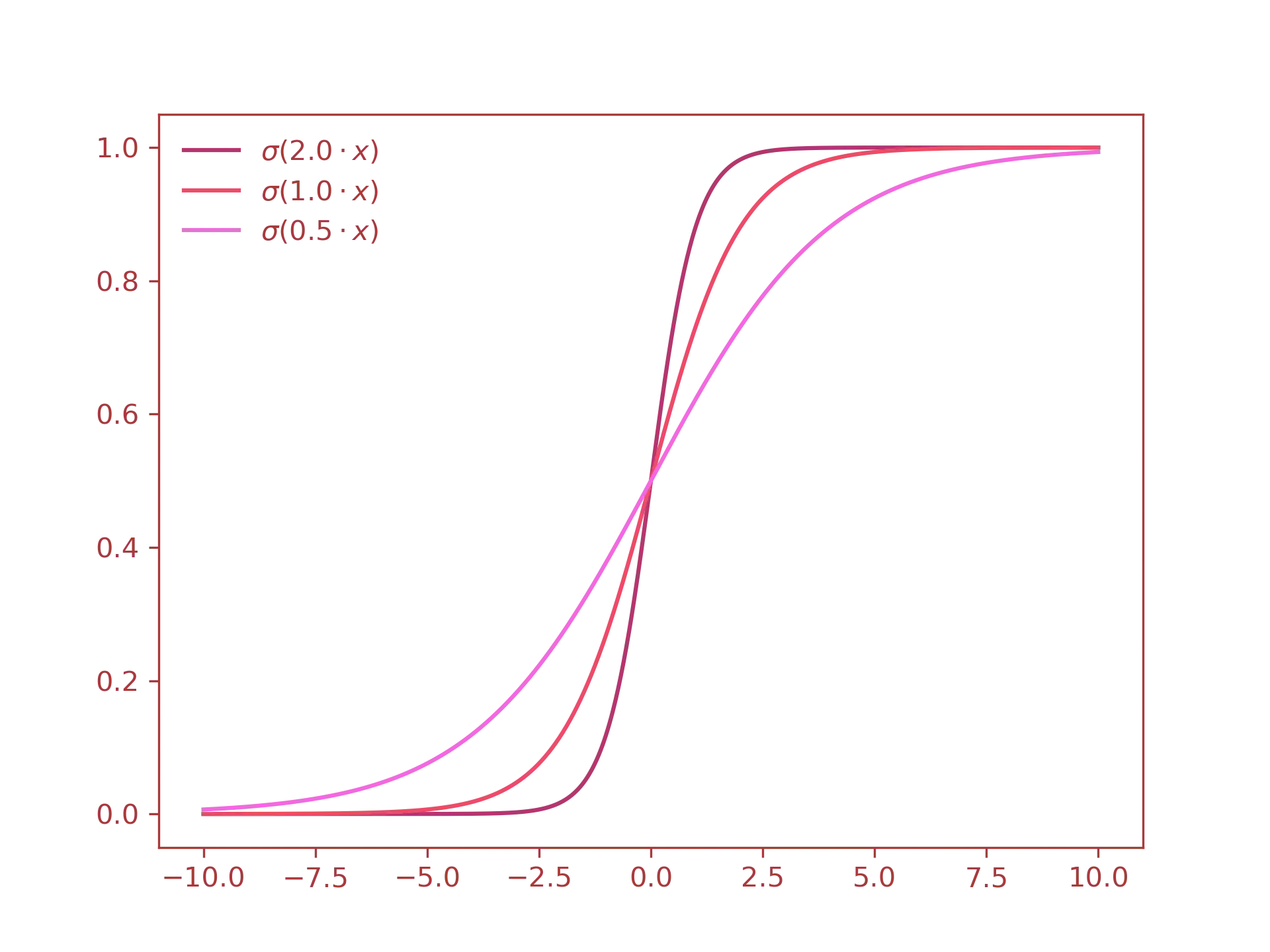
As you can see the effects are very limited. The main problem with this approach is that we have little to no control on how the neuron is being triggered. For example, what if we wanted the neuron to send the value $0$ when the input is equal to $1.0$? As you can see from the previous graph, changing the weight is not that effective. What you really want to do is to shift the whole curve to the right by a certain degree. In order to do that, you need to add the bias value to the sigmoid function. THis is exactly what happens to linear equations of the type $y = mx + q$ when you increase or decrease the $q$ parameter. Let us see this visually:
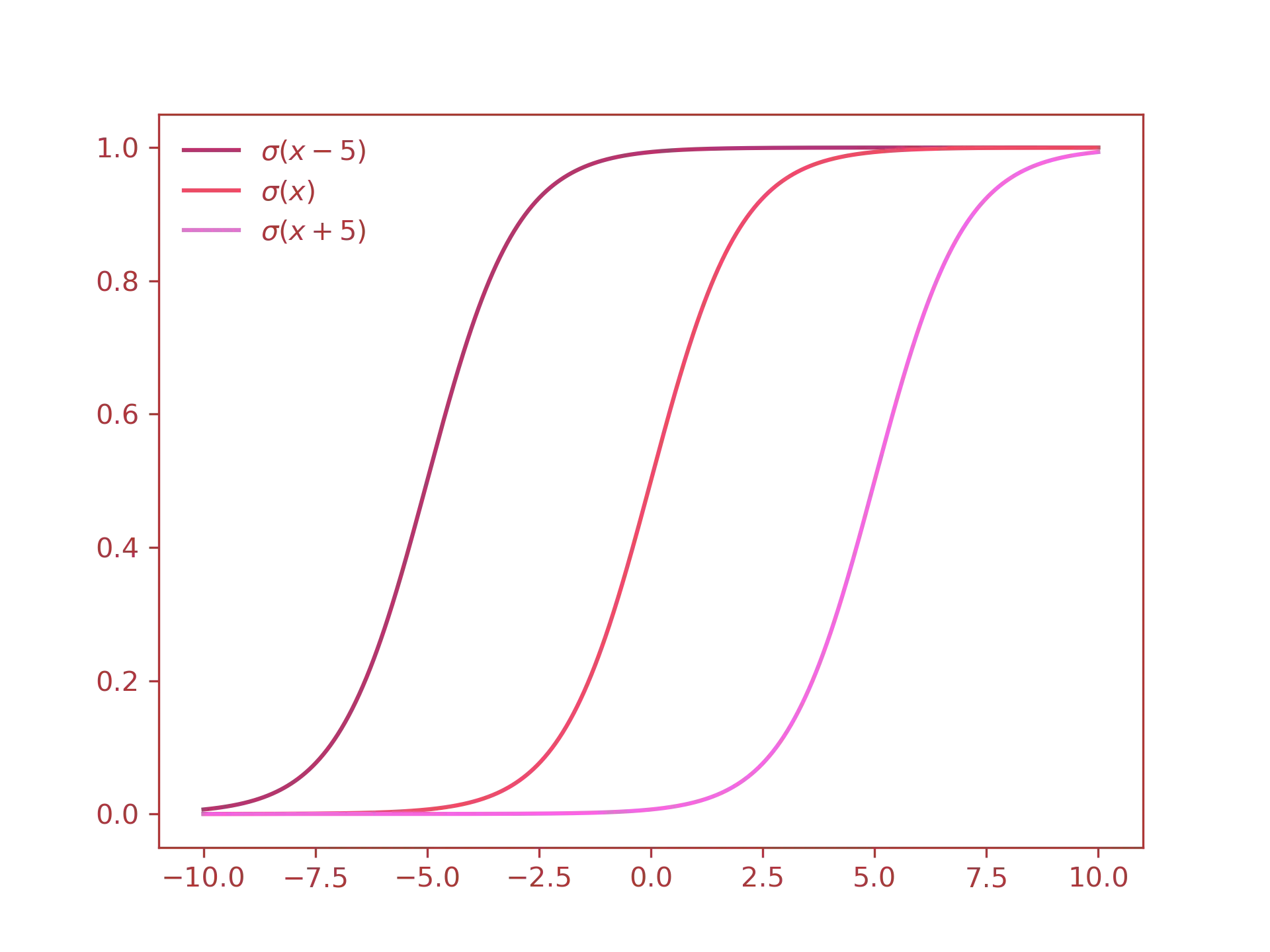
With a bias of $+5$, the input $1$ produces an output $\approx 0$.
In a neural network, the bias is added through another node called bias neuron, which has no input and produces always the same output, i.e.:
Keep in mind that bias is not always needed; nevertheless, the practical example of the next section will use it, since it allows the neural network to achieve a better accuracy rate.
Predict the XOR Logic Gate
In this section we will use everything we learned so far to write a neural network from scratch
to predict the output of a XOR logic gate. The neural network is written in Python using numpy
for linear algebra operations such as dot products, matrix transposition and summations.
Before anything else, let us see the truth table of the logical conjunction:
| $X_1$ | $X_2$ | $Y$ |
|---|---|---|
| 0 | 0 | 0 |
| 0 | 1 | 1 |
| 1 | 0 | 1 |
| 1 | 1 | 0 |
If we try to plot the outputs:
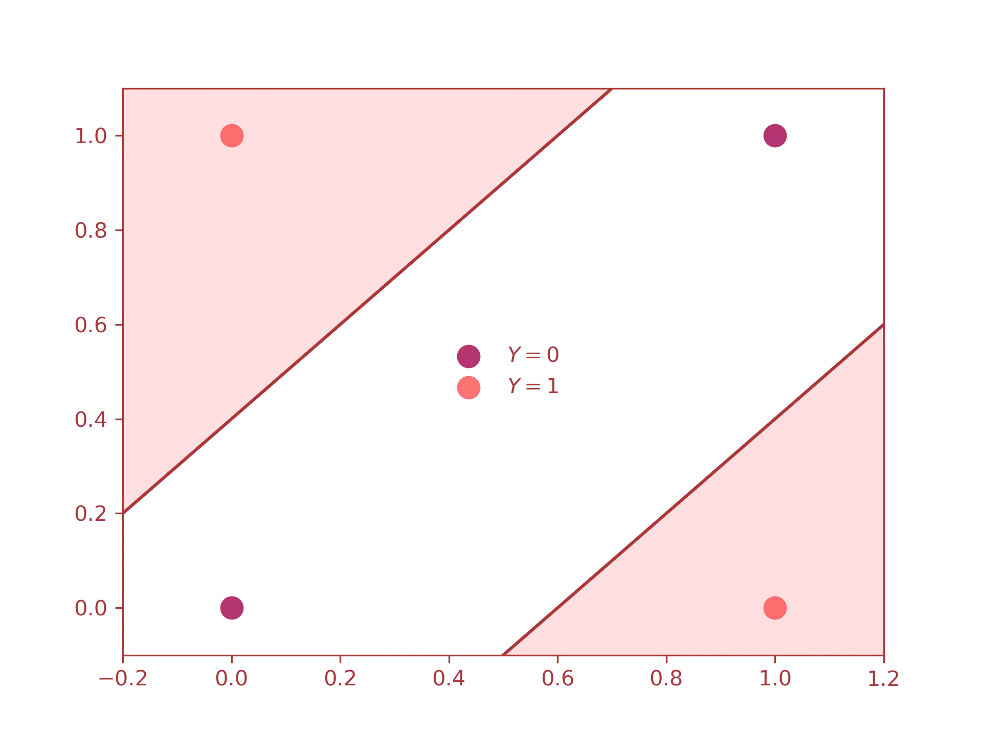
we can easily see that the inputs are not linearly separable, meaning that the neural network must separates the inputs using decisional regions. For the graph above, we notice that the active regions(i.e., the regions in red) are two, this means that our neural network will be modelled with two neurons in the hidden layer. Besides this, we also need two neurons for the input layer(one for each input) and one neuron for the output layer(since XOR produces just one output).
The final neural network will look like this:
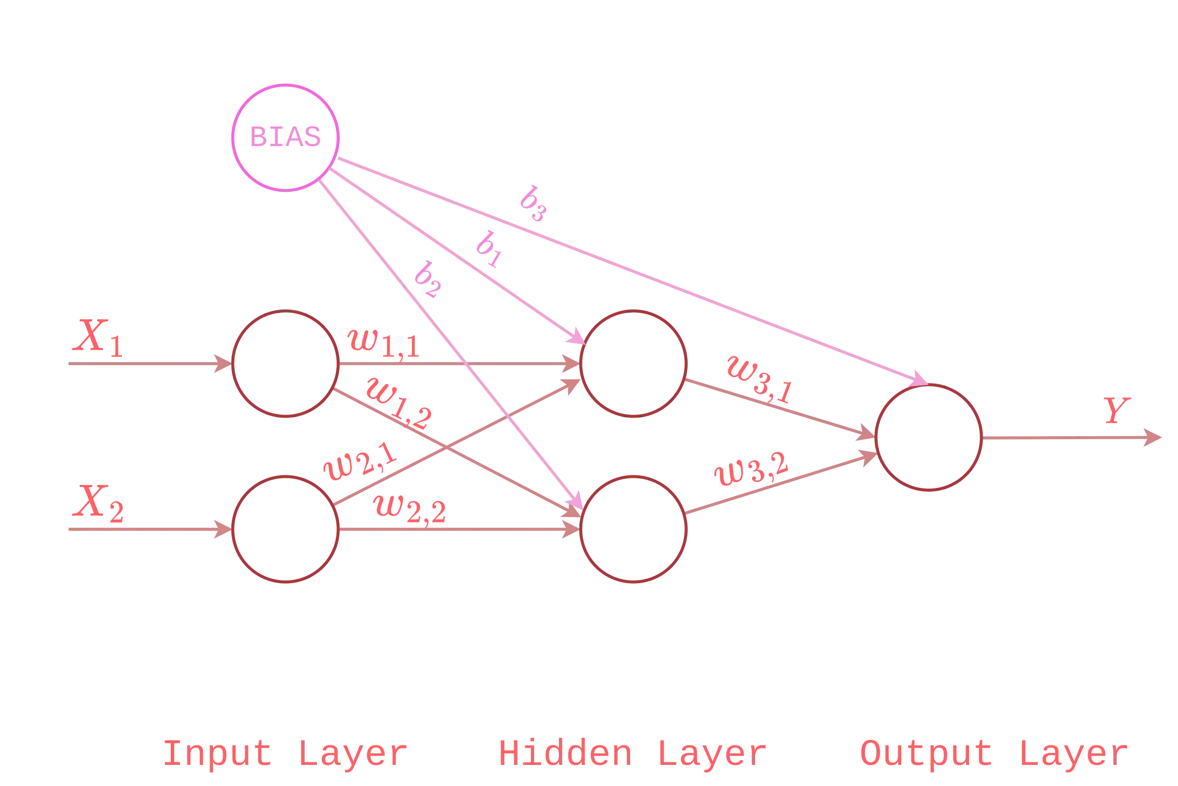
Let us start by defining a class XORNeuralNetwork as follows:
class XORNeuralNetwork:
    def __init__(self, inputs, expected_output):
        # Number of layers and neurons per layers
        self.input_layer_neurons = 2
        self.hidden_layer_neurons = 2
        self.output_layer_neurons = 1
        # Random weights and biases
        self.hidden_weight = np.random.rand(self.input_layer_neurons, self.hidden_layer_neurons)
        self.hidden_bias = np.random.rand(1, self.hidden_layer_neurons)
        self.output_weight = np.random.rand(self.hidden_layer_neurons, self.output_layer_neurons)
        self.output_bias = np.random.rand(1, self.output_layer_neurons)
        # Outputs from activation function
        self.hidden_layer_activation = None
        self.hidden_layer_output = None
        self.output_layer_activation = None
        self.predicted_output = None
        # Inputs and expected output
        self.input_vector = inputs
        self.expected_output = expected_output
in the constructor, we define the number of neurons per layer, the initial random weights and biases and the output from the learning process(empty by default). After that we implement the forward pass along with the sigmoid function:
# Activation function and its derivative
@staticmethod
def sigmoid(x):
    return 1 / (1 + np.exp(-x))

# Forward propagation
def feedforward(self):
    # Forward pass for hidden layer
    self.hidden_layer_activation = np.dot(self.input_vector, self.hidden_weight)
    self.hidden_layer_activation += self.hidden_bias
    self.hidden_layer_output = self.sigmoid(self.hidden_layer_activation)
    # Forward pass for output layer
    self.output_layer_activation = np.dot(self.hidden_layer_output, self.output_weight)
    self.output_layer_activation += self.output_bias
    self.predicted_output = self.sigmoid(self.output_layer_activation)
Basically, we compute the dot product between the weights and the inputs, then we add the bias, and finally we pass the result to the activation function. This process is repeated for the output layer.
After that we proceed to the backward pass:
@staticmethod
def sigmoid_derivative(x):
    return x * (1 - x)

# Backward propagation
def backpropagation(self):
    # Gradient descent of predicted output
    error_predicted_output = (self.expected_output - self.predicted_output)
    d_predicted_output = error_predicted_output * self.sigmoid_derivative(self.predicted_output)
    # Gradient descent of hidden layer
    error_hidden_layer = d_predicted_output.dot(self.output_weight.T)
    d_hidden_layer = error_hidden_layer * self.sigmoid_derivative(self.hidden_layer_output)
    # Update weights and biases of network
    self.output_weight += self.hidden_layer_output.T.dot(d_predicted_output)
    self.output_bias += np.sum(d_predicted_output, axis=0, keepdims=True)
    self.hidden_weight += self.input_vector.T.dot(d_hidden_layer)
    self.hidden_bias += np.sum(d_hidden_layer, axis=0, keepdims=True)

    return error_predicted_output
The last thing left to do is to define a train function
to repeat the learning process enough time to minimize the loss function.
def train(self, epoch=500):
    for i in range(epoch):
        progress = (i + 1) * 100 / epoch
        print(f"{int(progress)}% trained\r", end="")
        self.feedforward()
        self.backpropagation()
    print("")
As you can see I have set the epoch rate to $10,000$, this is a
quite large value, let us see how the error decrease over the iterations:
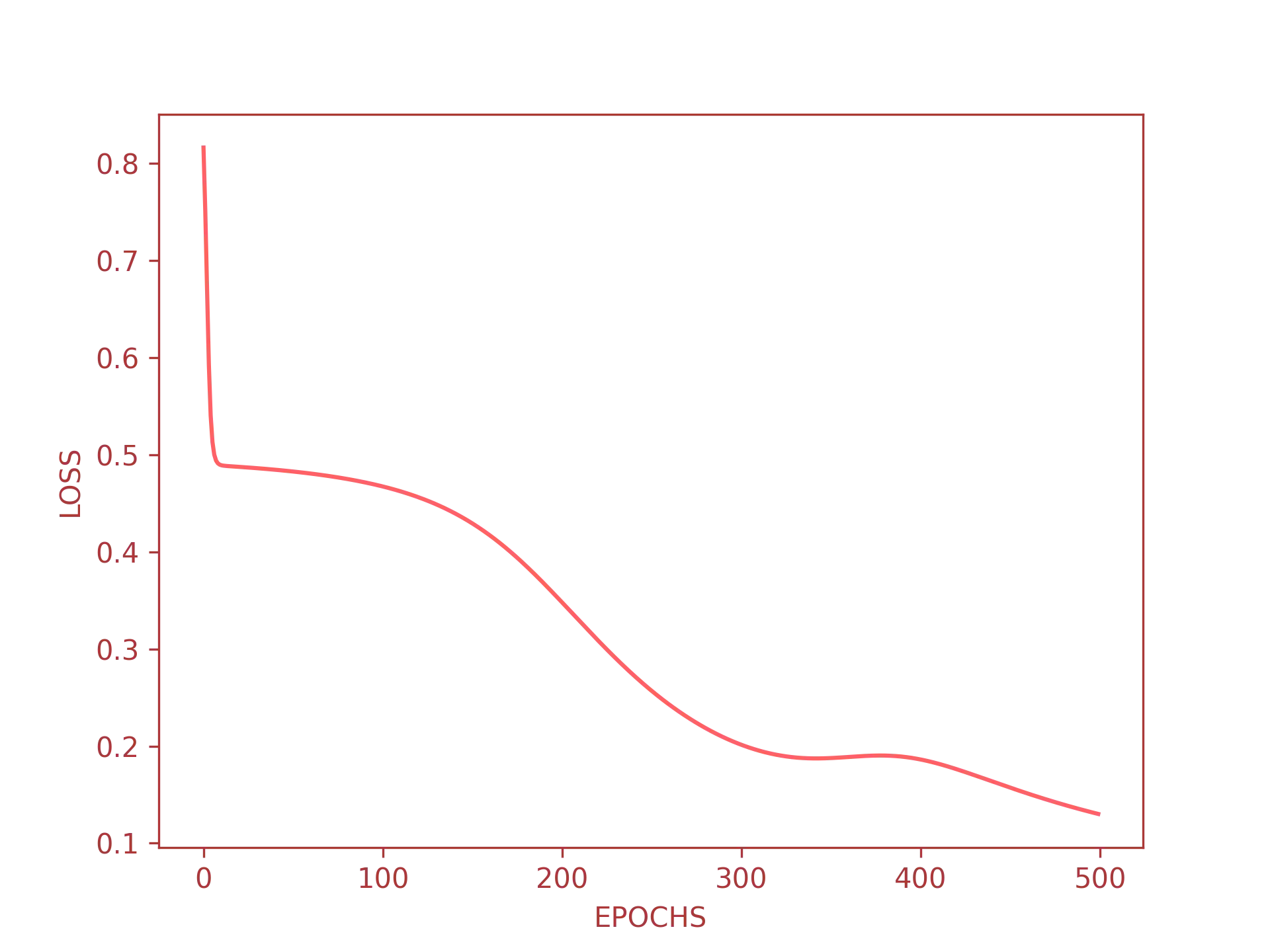
As you can see the error starts to approach an acceptable value after just 500 iterations. This means that an iteration rate of $\approx 5,000$ is more than enough for our neural network to predict good results.
Below, there is the complete source code. I have also included a driver code(i.e., the main function)
to test the trained neural network with user input.
import numpy as np

class XORNeuralNetwork:
    def __init__(self, inputs, expected_output):
        # Number of layers and neurons per layers
        self.input_layer_neurons = 2
        self.hidden_layer_neurons = 2
        self.output_layer_neurons = 1
        # Random weights and biases
        self.hidden_weight = np.random.rand(self.input_layer_neurons, self.hidden_layer_neurons)
        self.hidden_bias = np.random.rand(1, self.hidden_layer_neurons)
        self.output_weight = np.random.rand(self.hidden_layer_neurons, self.output_layer_neurons)
        self.output_bias = np.random.rand(1, self.output_layer_neurons)
        # Outputs from activation function
        self.hidden_layer_activation = None
        self.hidden_layer_output = None
        self.output_layer_activation = None
        self.predicted_output = None
        # Inputs and expected output
        self.input_vector = inputs
        self.expected_output = expected_output

    # Activation function and its derivative
    @staticmethod
    def sigmoid(x):
        return 1 / (1 + np.exp(-x))

    @staticmethod
    def sigmoid_derivative(x):
        return x * (1 - x)

    # Forward propagation
    def feedforward(self):
        # Forward pass for hidden layer
        self.hidden_layer_activation = np.dot(self.input_vector, self.hidden_weight)
        self.hidden_layer_activation += self.hidden_bias
        self.hidden_layer_output = self.sigmoid(self.hidden_layer_activation)
        # Forward pass for output layer
        self.output_layer_activation = np.dot(self.hidden_layer_output, self.output_weight)
        self.output_layer_activation += self.output_bias
        self.predicted_output = self.sigmoid(self.output_layer_activation)

    # Backward propagation
    def backpropagation(self):
        # Gradient descent of predicted output
        error_predicted_output = (self.expected_output - self.predicted_output)
        d_predicted_output = error_predicted_output * self.sigmoid_derivative(self.predicted_output)
        # Gradient descent of hidden layer
        error_hidden_layer = d_predicted_output.dot(self.output_weight.T)
        d_hidden_layer = error_hidden_layer * self.sigmoid_derivative(self.hidden_layer_output)
        # Update weights and biases of network
        self.output_weight += self.hidden_layer_output.T.dot(d_predicted_output)
        self.output_bias += np.sum(d_predicted_output, axis=0, keepdims=True)
        self.hidden_weight += self.input_vector.T.dot(d_hidden_layer)
        self.hidden_bias += np.sum(d_hidden_layer, axis=0, keepdims=True)

        return error_predicted_output

    def train(self, epoch=500):
        for i in range(epoch):
            progress = (i + 1) * 100 / epoch
            print(f"{int(progress)}% trained\r", end="")
            self.feedforward()
            self.backpropagation()
        print("")

    def predict(self, data):
        # Forward pass for hidden layer
        self.hidden_layer_activation = np.dot(data, self.hidden_weight)
        self.hidden_layer_activation += self.hidden_bias
        self.hidden_layer_output = self.sigmoid(self.hidden_layer_activation)
        # Forward pass for output layer
        self.output_layer_activation = np.dot(self.hidden_layer_output, self.output_weight)
        self.output_layer_activation += self.output_bias
        self.predicted_output = self.sigmoid(self.output_layer_activation)

        return self.predicted_output


def main():
    truth_table = np.array([[0, 0], [0, 1], [1, 0], [1, 1]])
    expected_output = np.array([[0, 1, 1, 0]]).T
    nn = XORNeuralNetwork(truth_table, expected_output)

    # Train the network
    nn.train(epoch=5000)

    try:
        while True:
            # Ask user for two values
            x = int(input("Enter x: "))
            y = int(input("Enter y: "))
            input_vector = np.array([[x, y]])

            # predict XOR of x_1 and x_2 using neural network
            prediction = nn.predict(input_vector)

            print(f"({x} ^ {y}) = {prediction[0][0]}")

    except (KeyboardInterrupt, ValueError):
        print("Bye")
        exit(0)


if __name__ == "__main__":
    main()
Let us try it.
(venv) marco@archtop $> python3 main.py
100% trained
Enter x: 0
Enter y: 0
(0 ^ 0) = 0.019274204763050903
Enter x: 0
Enter y: 1
(0 ^ 1) = 0.983340815029345
Enter x: 1
Enter y: 0
(1 ^ 0) = 0.9833791938260293
Enter x: 1
Enter y: 1
(1 ^ 1) = 0.017250301094216512
Enter x: q
Bye
It works! As you can see the prediction is quite good and the output is very close to the expected value.