Continuous Functions

The standard definition of continuity usually presented in elementary mathematics texts describes a function as continuous if its graph can be traced “without lifting the pencil from the paper. Although this idea provides an intuitive starting point from absolute beginners, it is neither precise nor reliable for more advanced or non-elementary functions. Therefore, in this guide, we will examine continuous functions from both analytical and topological perspectives. We will also explore how to handle points or regions in the domain where a function ceases to be continuous.

Definition using limits

The first definition of continuity relies on the $\epsilon$-$\delta$ definition of limits. Formally:

Let $f : A \subseteq \mathbb{R} \to \mathbb{R}$ be a function and let $x_0 \in A$ an accumulation point for $A$. The function $f$ is continuous at $x_0$ if $$ \lim_{x \to x_0} f(x) = f(x_0) $$

In other words, a function is continuous at $x_0$ if the limit of $f(x)$ as $x$ tends to $x_0$ is equal to the value of the function at that point. From this definition, we obtain that:

A function $f : A \subseteq \mathbb{R} \to \mathbb{R}$ is continuous on $A$ if it is continuous $\forall x \in A$.

Let’s look at a simple example. Given the function:

$$ f(x) = \cos(x) $$

and the point $x_0 = 0$, we have that:

$$ \lim_{x \to 0} \cos(x) = 1 = \cos(0) $$

Thus, $\cos(x)$ is continuous on $x = 0$ (and, in fact, $\forall x \in \mathbb{R}$).

Topological definition

Another way to define continuity is from a topological perspective, where instead of defining it in terms of a metric concept such as distance, we formalize it using open sets.

Let $(X, \tau_X)$ and $(Y, \tau_Y)$ two topological spaces. A function $f : X \to Y$ is continuous if the preimage of every open subsets in the codomain is also an open subset in the domain.

In other words, $f$ is continuous if, for all $V \subseteq Y$, the preimage: $$ f^{-1}(V) := \{ x \in X : f(x) \in V \} $$ is also an open subsets in $X$. That is:

$$ \forall V \in \tau_Y \implies f^{-1}(V) \in \tau_X $$

In the Euclidean space $\mathbb{R}$ equipped with the standard topology, open sets can be expressed as unions of open intervals. Thus, if we take an open neighborhood $$ V = (f(x_0) - \epsilon, f(x_0) + \epsilon) $$

of $f(x_0)$ in the codomain, then its preimage $f^{-1}(V)$ will contain an open neighborhood $$ U = (x_0 - \delta, x_0 + \delta) $$ of $x_0$ in the domain.

Let’s look at a practical example. Let $f : \mathbb{R} \to \mathbb{R}$ be the function defined by $f(x) = x^2$ and let $V = (1,4)$ be an open interval in the codomain $\mathbb{R}$. Its preimage is the set defined by: by the set:

$$ \begin{aligned} f^{-1}((1,4)) &= \{ x \in \mathbb{R} : 1 < x^2 < 4 \}\\ &= (-2, -1) \cup (1,4) \end{aligned} $$

Which is the union of two open intervals and is therefore an open set in $\mathbb{R}$.

Discontinuities

A point $x_0$ is called a point of discontinuity of a function $f$ if the $f$ is defined at $x_0$ but it is not continuous there. The types of discontinuities that we will study in this guides are:

• Jump discontinuity;
• Infinite discontinuity;
• Removable discontinuity.

Let’s see them in details.

Jump discontinuities

A jump discontinuity is a type of discontinuity where both the left-hand and right-hand limits exist but they are not equal. That is:

$$ \lim_{x \to x_0^-} f(x) = L_1, \ \ \lim_{x \to x_0^+} f(x) = L_2 $$

where: $$ L_1, L_2 \in \mathbb{R}, L_1 \neq L_2 $$

For example, given:

$$ f(x) = \begin{cases} x + 1, & x < 1\\ \frac{x}{2}, & x \geq 1 \end{cases} $$

We have the following jump at $x=1$:

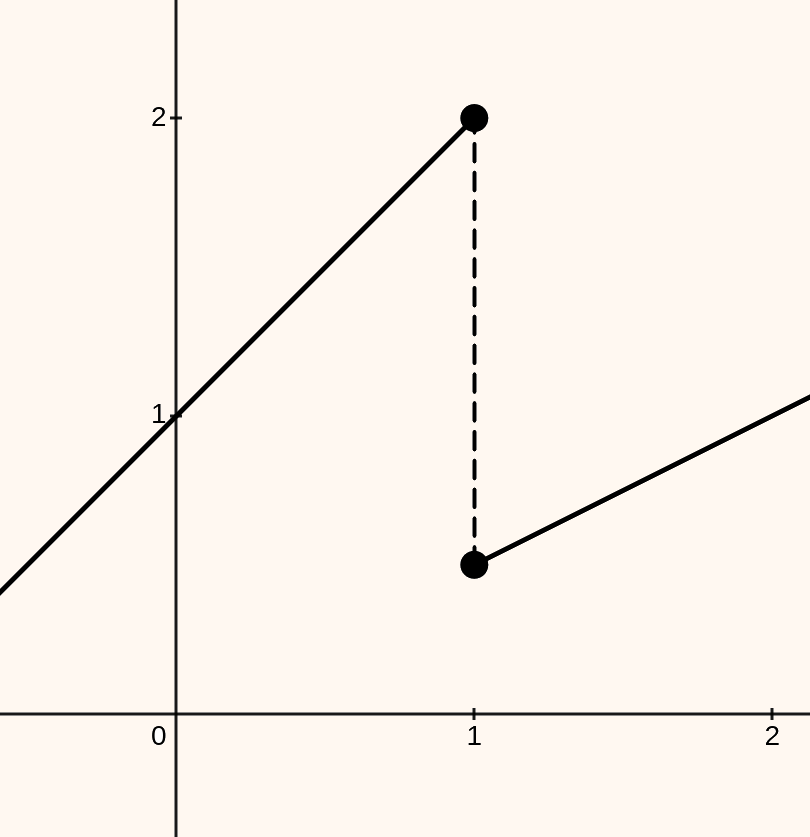
In fact, if we evaluate the left-hand and the right-hand limits at $x=1$, we obtain: $$ \lim_{x \to 1^-} f(x) = \lim_{x \to 1^-} (x + 1) = 2 $$

On the other hand, from the right:

$$ \lim_{x \to 1^+} f(x) = \lim_{x \to 1^+} \frac{x}{2} = \frac{1}{2} $$

As you can see from the previous picture, the graph “jumps” from $2$ down to $\frac{1}{2}$. The size of the jump is therefore:

$$ | L_2 - L_1 | = \left|\frac{1}{2} - 2\right| = \frac{3}{2} $$

Infinite discontinuities

An infinity discontinuity is a type of discontinuity where at least one of the one-sided limits as $x \to x_0$ is diverges to $\pm \infty$. That is:

$$ \lim_{x \to x_0^-} f(x) = \pm \infty \ \ \vee \ \ \lim_{x \to x_0^+} f(x) = \pm \infty $$

For example, let’s consider the following function, which represents a rectangular hyperbola:

$$ f(x) = \frac{1}{x} $$

has a discontinuity at $x=0$. In fact:

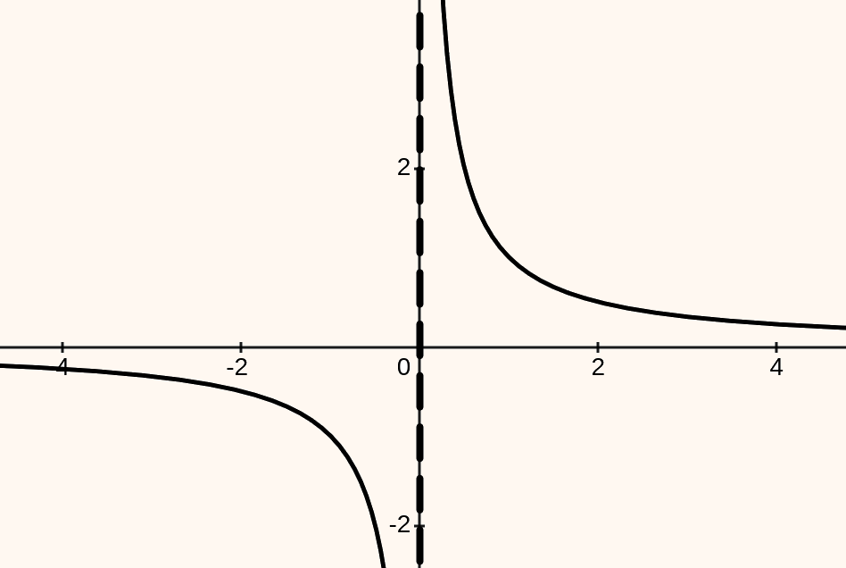
As you can see from the previous graph, from the right, the function rises to $+\infty$, while from the left, it decreases to $-\infty$. Let’s prove this analytically:

$$ \lim_{x \to 0^-} \frac{1}{0^-} = -\infty $$

On the other hand:

$$ \lim_{x \to 0^+} \frac{1}{0^+} = +\infty $$

Removable discontinuity

The last type of discontinuity we will study on this guide is called “removable discontinuity”. It occurs when the limit as $x \to x_0$ exists and it’s finite but it is not equal to $f(x_0)$. That is:

$$ \begin{aligned} &\lim_{x \to x_0^-} f(x) = \lim_{x \to x_0^-} f(x) = L \in \mathbb{R},\\ &f(x_0) \neq L \end{aligned} $$

It is called removable because the function can be redefined to obtain a new continuous function. We do this by setting: $$ f(x_0) = L $$

Let’s see an example. Given: $$ f(x) = \frac{\sin(x)}{x} $$

Its domain is $\mathbb{R} \setminus \{ 0 \}$. If we try to compute the limit as $x \to 0$ we obtain:

$$ \lim_{x \to 0} = \frac{\sin(x)}{x} = 1 $$

However, the function is not defined at $x_0 = 0$. To remove this discontinuity, we define a continuous extension of the original function by setting $f(0) = 1$. With this definition, the function becomes continuous at $x=0$.