Limits of Sequences and Functions
In analysis, a limit is a fundamental concept that is used to study the behavior of a function as its argument approaches a given value $x_0$ or tends to infinity. Limits can be defined for both sequences and functions, in the former case they are particularly useful because they allow us to determine whether the sequence converges to a value or not.
Let’s start with the definition of the limit of a sequence.
Limit of a sequence
First of all, let’s recall that a sequence $$ a : \mathbb{N} \to \mathbb{R} $$
is a function whose domain is the set of natural numbers. We usually denote sequences using $(a_n)_{n \in \mathbb{N}}$ or $a_n$ where $n$ denotes their index.
We say that the sequence $a_n$ tends to the limit $L \in \mathbb{R}$ as $n \to +\infty$ and we write: $$ \lim_{n \to +\infty} a_n = L $$
if and only if $\forall \epsilon > 0, \ \ \exists N \in \mathbb{N}$ such that
$$ \forall n \geq N, \ \ |a_n - L| < \epsilon $$
Okay, let’s try to decipher what’s going on here: we first choose an arbitrary positive number $\epsilon$ which in turn determines a natural number $N$. Then, we require that the distance between any term $a_n$ of the sequence and $L$ (the value of the limit) must be strictly less than $\epsilon$ after we crossed a certain threshold $N$. In other words, we require that from some index $N$ onward, all the terms of the sequence must remain arbitrarily close to $L$.
We can represent this concept with the following diagram:
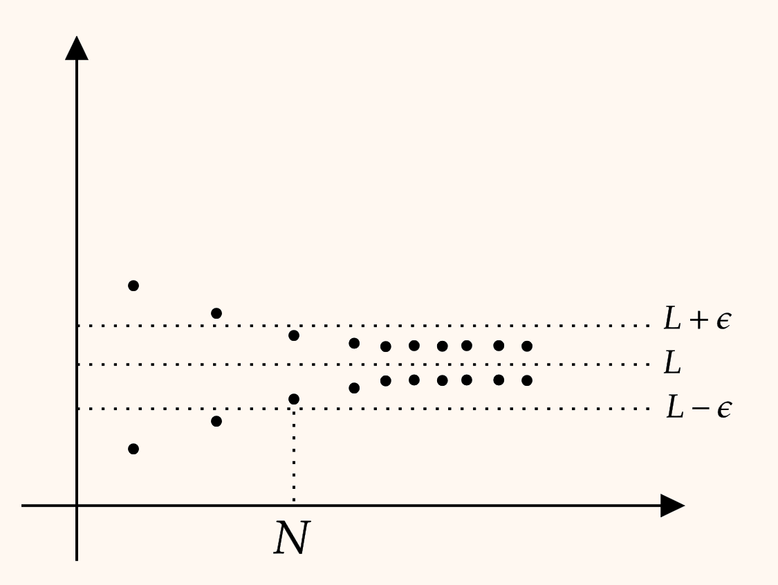
Do note that this diagram represents only one particular “strip” (i.e., the height determined by $\epsilon$), but the definition states that this must work $\forall \epsilon > 0$.
Let’s try to apply the definition to an actual example. For instance, we want to prove that: $$ \lim_{n \to +\infty} \frac{2n+1}{n+2} = 2 $$
In other words, we want to prove that, $\forall \epsilon > 0$, there is a natural number $N$ such that, $\forall n \geq N$, the following inequality holds:
$$ \left| \frac{2n+1}{n+2} - 2 \right| < \epsilon $$
Let’s work out the expression inside the absolute value first:
$$ \frac{2n+1}{n+2} - 2 = \frac{2n+ 1 - 2(n+2)}{n+2} = \frac{2n + 1 - 2n - 4}{n+2} = \frac{-3}{n+2} $$
The inequality becomes:
$$ \left| \frac{-3}{n+2} \right| < \epsilon \iff \frac{3}{n+2} < \epsilon $$
Now let’s isolate $n$ (since $n \in \mathbb{N}$, it’s always non-negative):
$$ 3 < \epsilon (n+2) \implies \frac{3}{\epsilon} < n + 2 \implies n > \frac{3}{\epsilon} - 2 $$
This means that our threshold is $N > \frac{3}{\epsilon} - 2$. Let’s choose a value that satisfies this constraint, let $N = \lceil \frac{3}{\epsilon} \rceil$ and now let’s prove that the definition holds. Let $\epsilon > 0$; thus, for every $n \geq N$, we have that $n+2 \geq N + 2 > \frac{3}{\epsilon}$. From there, we can notice that:
$$ \left| \frac{2n+1}{n+2} -2 \right| = \frac{3}{n+2} < \epsilon $$
Therefore: $$ \left| \frac{2n+1}{n+2} -2 \right| < \epsilon \quad \forall n \geq N $$
Since the definition holds, the sequence converges to the value $2$. In fact, this example allows us to state that:
- If $\lim_{n \to +\infty} a_n = L \in \mathbb{R}$, then the sequence is convergent;
- If $\lim_{n \to +\infty} a_n = \pm \infty$, then the sequence is divergent.
Limit of a function
Let’s now extend the notion of limit to real-valued functions. In order to do this, we will first need a couple of topological prerequisites.
Given a real number $x_0 \in \mathbb{R}$, a neighborhood $I$ of $x_0$ is any open interval centered at $x_0$ with radius $\delta > 0$. That is: $$ I(x_0) = (x_0 - \delta, x_0 + \delta), \ \ \delta > 0 $$
In other words, a neighborhood of a point is any open interval containing real numbers sufficiently close to that point.
Now the other prerequisite:
Let $A \subseteq \mathbb{R}$ be a non-empty subset. A point $x_0 \in \mathbb{R}$ is an accumulation point for $A$ if every neighborhood $I(x_0)$ of $x_0$ contains at least an element $x \in A$ that is different from $x_0$ itself. That is: $$ \forall I(x_0), \exists x \in A : x \in I(x_0) \setminus \{ x_0 \} $$
In other words, this means that near $x_0$ we can always find elements of $A$ which are different from $x_0$.
This last definition is essential for the topological definition ($\epsilon$-$\delta$) of limits of functions. In fact, a limit of a function at $x_0$ is meaningful only when $x_0$ is an accumulation point of the domain of the function.
Let $$ f : A \subseteq \mathbb{R} \to \mathbb{R} $$
be a real-valued function and let $x_0 \in \mathbb{R}$ be an accumulation point of $A$. We say that the function $f$ tends to the real value $L$ as $x$ tends to $x_0$, and we write:
$$ \lim_{x \to x_0} f(x) = L \in \mathbb{R} $$
If and only if $\forall \epsilon > 0, \exists \delta(\epsilon) > 0$ such that, $\forall x \in A \setminus \{ x_0 \}$:
$$ 0 < | x - x_0 | < \delta \implies | f(x) - L | < \epsilon $$
Let’s analyze this definition step by step. First of all, although both $\epsilon$ and $\delta$ denote two positive numbers, they play different roles in the definition: given any $\epsilon > 0$, we must be able to find a corresponding $\delta > 0$; this means that the value of $\delta$ is determined by the choice of $\epsilon$. In particular, $\epsilon$ represents a distance on the $y$-axis, while $\delta$ represents a distance on the $x$-axis.
On the second part, instead, the inequality: $$ | x - x_0 | < \delta $$
tells us that for any element $x \in A, x \neq x_0$ of the $x$-axis, the distance between $x$ and $x_0$ must be less than $\delta$. Additionally, we express the fact that $x \neq x_0$ with the following inequality:
$$ 0 < | x - x_0 | $$
Therefore, we are considering points $x$ in the punctured neighborhood defined by:
$$ (x_0 - \delta, x_0 + \delta) \setminus \{ x_0 \} $$
If $x$ satisfies these conditions, then the corresponding value $f(x)$ must be sufficiently close to $L$. That is:
$$ | f(x) - L | < \epsilon $$
This means that the distance between the $y$-value of $f(x)$ and the real value $L$ is less than $\epsilon$. In other words, the definition states that no matter how small we choose $\epsilon$, we can always find a corresponding $\delta$ on the $x$-axis such that every $x$ sufficiently close to $x_0$ (but different from it) produces a value $f(x)$ sufficiently close to $L$. If this condition holds $\forall \epsilon > 0$, then we say that the limit exists and that it is equal to $L$.
To visualize what the definition is trying to convey, take a look at the following diagram:
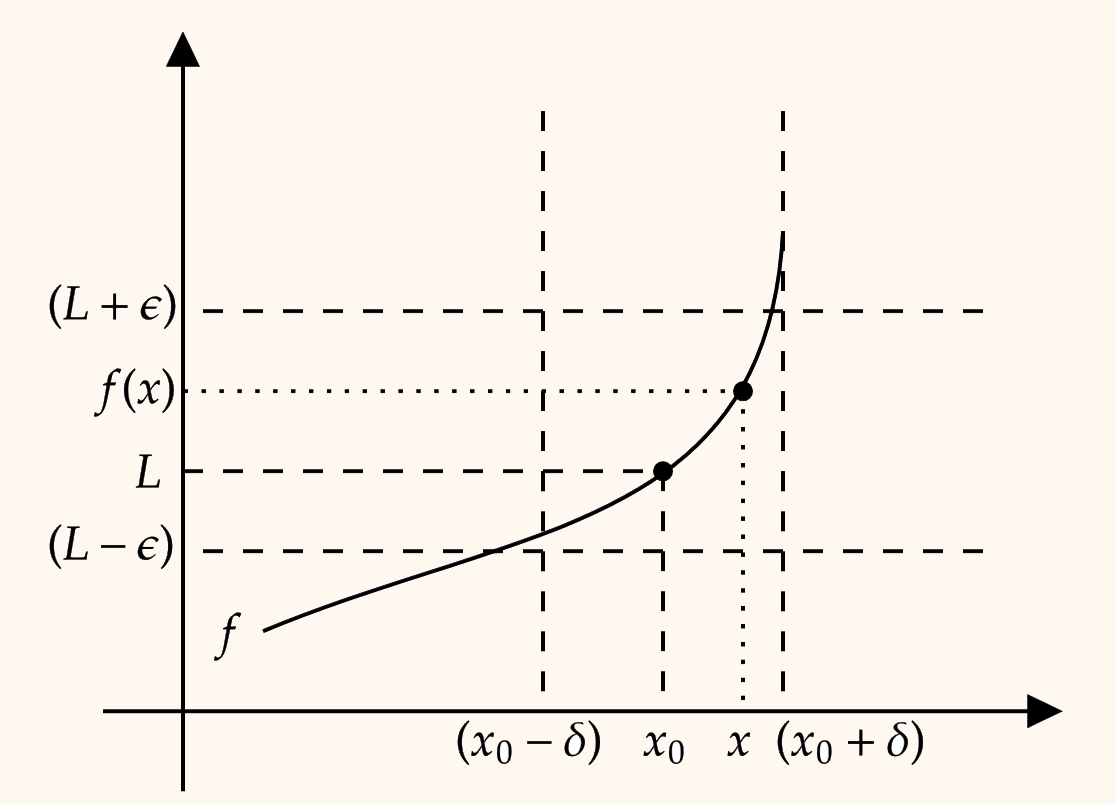
Again, let’s try to analyze it step by step. First, we choose a positive $\epsilon$, which determines the interval $(L - \epsilon, L + \epsilon)$ on the $y$-axis. We then choose a corresponding $\delta > 0$ which determines the interval $(x_0 - \delta, x_0 + \delta)$ on the $x$-axis. Then, for any $x \in A \setminus \{ x_0 \}$, we have that $|x - x_0 | < \delta$; that is, the value $x$ lies inside the $\delta$-neighborhood of $x_0$ (while being different from $x_0$). By evaluating the function $y = f(x)$ we obtain a corresponding value on the $y$-axis and, according to the definition, this value must satisfy the condition $|f(x) - L | < \epsilon$. In other words, the image of $f$ evaluated at $x$ must lie inside the interval $(L - \epsilon, L + \epsilon)$.
If this constraint is met $\forall x \in A \setminus \{ x_0 \}$ sufficiently close to $x_0$ and, $\forall \epsilon > 0$ there exists a corresponding $\delta > 0$, then we can write that: $$ \lim_{x \to x_0} f(x) = L $$
and we say that the limit is convergent to $L$. Depending on whether $x_0$ and $L$ are numbers or $\pm \infty$, we can configure the following three variants of the general definition.
1. Divergent limit at a finite point
Given the function $$ f : A \subseteq \mathbb{R} \to \mathbb{R} $$
we say that $$ \lim_{x \to x_0} f(x) = +\infty $$
If and only if $\forall k > 0, \exists \delta(k) > 0$ such that $$ 0 < | x - x_0 | < \delta \implies f(x) > k $$
Similarly, we say that $$ \lim_{x \to x_0} f(x) = -\infty $$
if and only if $\forall k > 0, \exists \delta(k) > 0$ such that $$ 0 < | x - x_0 | < \delta \implies f(x) < -k $$
2. Convergent limit at infinity
Given the function $$ f : A \subseteq \mathbb{R} \to \mathbb{R} $$
we say that
$$ \lim_{x \to +\infty} f(x) = L \in \mathbb{R} $$
if and only if $\forall \epsilon > 0, \exists k(\epsilon) > 0$ such that $$ x > k \implies | f(x) - L | < \epsilon $$
Similarly, we say that $$ \lim_{x \to -\infty} f(x) = L \in \mathbb{R} $$
if and only if $\forall \epsilon > 0, \exists k(\epsilon) > 0$ such that $$ x < -k \implies | f(x) - L | < \epsilon $$
3. Divergent limit at infinity
Given the function $$ f : A \subseteq \mathbb{R} \to \mathbb{R} $$
we say that
$$ \lim_{x \to +\infty} f(x) = +\infty $$
if and only if $\forall h >0, \exists k(h) > 0$ such that $$ x > k \implies f(x) > h $$
The structure of the definition remains identical for the other signs as well, with the only thing changing being the directions of the inequalities and the signs of the boundary variables $h$ and $k$.
As a matter of example, let’s see the definition of $$ \lim_{x \to +\infty} f(x) = -\infty $$
This limit exists if and only if $\forall h > 0, \exists k(h) > 0$ such that $$ x > k \implies f(x) < -h $$
This means that the $x$ variable tends to the right but, unlike the previous case where the function rises towards the top ($+\infty$), the function decreases towards the bottom ($-\infty$). You can easily derive all the other cases by following this reasoning.
Evaluating a limit
Now that it’s clear what it means to take the limit of a sequence or of a function, let’s try to evaluate them. From a practical point of view, solving, evaluating and calculating a limit means evaluating the function on $x_0$, work out the algebra (if any) and then determining whether the limit converges to a finite value $L$ or to $\pm \infty$.
For example:
$$ \lim_{x \to 5} x^2 - 6x + 8 = 3 $$
As you can see, evaluating this limit is equivalent to replacing $x$ with $5$. Naturally, we can do the same for a limit for $x \to \pm \infty$:
$$ \lim_{x \to \infty} \frac{1}{x^2} = 0 $$
More generally, we need to keep in mind the following rules when evaluating such limits:
$$ \lim_{x \to \pm \infty} x^n = +\infty, \ n > 0 $$
$$ \lim_{x \to \pm \infty} \frac{1}{x^n} = 0, \ n > 0 $$
$$ \lim_{x \to +\infty} \sqrt{x} = +\infty $$
$$ \lim_{x \to + \infty} e^x = +\infty \ \ \text{and} \ \ \lim_{x \to -\infty} e^x = 0 $$
Instead, for a polynomial $$ P(x) = a_n x^n + \dotsc + a_1 x + a_0 $$
the highest-degree term and the parity of $n$ determine the sign of the limit as $x \to \pm \infty$. In particular:
$$ \lim_{x \to +\infty} P(x) = \begin{cases} + \infty &a_n > 0\\ - \infty &a_n < 0 \end{cases} $$
And $$ \lim_{x \to -\infty} P(x) = \begin{cases} +\infty &a_n > 0, \ \ n \text{ is even}\\ -\infty &a_n < 0, \ \ n \text{ is even}\\ -\infty &a_n > 0, \ \ n \text{ is odd}\\ +\infty &a_n < 0, \ \ n \text{ is odd} \end{cases} $$
Moreover, given two functions $f(x)$ and $g(x)$ such that $\lim_{x \to x_0} f(x) = L_1$ and $\lim_{x \to x_0} g(x) = L_2$ with $L_1, L_2 \in \mathbb{R}$, we have the following algebraic properties:
- Sum: $\lim_{x \to x_0} f(x) \pm g(x) = L_1 \pm L_2$;
- Product: $\lim_{x \to x_0} f(x) \cdot g(x) = L_1 \cdot L_2$;
- Product by a constant: $\lim_{x \to x_0} c \cdot f(x) = c \cdot L_1$ with $c \in \mathbb{R}$;
- Power: $\lim_{x \to x_0} [f(x)]^{g(x)} = L_1^{L_2}$ with $L_1 > 0$.
Indeterminate forms
When evaluating a limit using the techniques introduced in the previous section, we may encounter combinations for which knowing the individual limits of the functions is not enough to determine if the overall limit converges or not. It’s the case of following seven indeterminate forms:
$$ [ +\infty - \infty], \ \ [0 \cdot \infty], \ \ \left[ \frac{0}{0} \right], \ \ \left[ \frac{\infty}{\infty} \right], \ \ [ 1^{\infty} ], \ \ [0^0 ], \ \ [\infty^0 ] $$
Let’s look at an example:
$$ \lim_{x \to +\infty} \frac{3x^2 + 5x + 2}{2x^2 + 3x + 1} = \left[ \frac{\infty}{\infty} \right] $$
The issue is that there is no simple way to determine which of the two functions tends to infinity “faster”. In such cases, there is a whole range of techniques, theorems and algebraic manipulations to determine whether the limit exists or not. The technique we will discuss in this guide is to factor out the highest power of $x$ from the numerator and denominator.
In other words:
$$ \lim_{x \to +\infty} \frac{x^2(3 + \frac{5}{x} + \frac{1}{x^2})}{x^2(2 + \frac{3}{x} + \frac{1}{x^2})} $$
And since the fractions ($\frac{5}{x}, \frac{1}{x^2}$, $\frac{3}{x}$) tend to zero as $x \to +\infty$ and the two $x^2$ cancel each other out, we obtain:
$$ \lim_{x \to +\infty} \frac{3 + 0 + 0}{2 + 0 + 0} = \frac{3}{2} $$
If we instead tried to evaluate the following limit with the same technique:
$$ \lim_{x \to +\infty} \frac{2x^3 + 5x}{x+1} = \left[ \frac{\infty}{\infty} \right] = \frac{x^3(2 + \frac{5}{x^2})}{x(1 + \frac{1}{x})} $$
In this case, $\frac{x^3}{x} = x^2$ and the two fractions tend to zero as $x \to +\infty$, therefore:
$$ \lim_{x \to +\infty} \frac{x^2(2 + 0)}{1 + 0} = +\infty $$
Last example:
$$ \lim_{x \to +\infty} \frac{x+1}{x^2+3} = \left[ \frac{\infty}{\infty} \right] = \lim_{x \to +\infty} \frac{x(1 + \frac{1}{x})}{x^2(1 + \frac{3}{x^2})} $$
In this case, $\frac{x}{x^2} = \frac{1}{x}$ and the two fractions tend to zero as $x \to +\infty$, therefore:
$$ \lim_{x \to +\infty} \frac{1}{x(1 + 0)} = 0 $$
There are obviously many other ways to solve these indeterminate forms, such as l’Hôpital’s rule or Taylor polynomials, but we won’t cover them in this guide.
One-sided limits
In some circumstances, the limit of a function may not exist; that is, it is not convergent to a real number nor diverges to $\pm \infty$. In such cases, it is useful to study the behavior of the function from a different standpoint. In particular, we would like to know what happens when we approach a certain point from the left or the right of the function.
In order to do this, we need to introduce the notions of right-sided limits and left-sided limits. For both of them, the definition is the same. The only difference lies in the choice of the neighborhoods and therefore in their topology.
Right-sided limit
Given the function $$ f : A \subseteq \mathbb{R} \to \mathbb{R} $$
and $x_0$ a right-sided accumulation point of $A$, we define the limit of $f(x)$ as $x$ tends to $x_0^{+}$ from the right as: $$ \lim_{x \to x_0^{+}} f(x) = L^+ $$
if and only if $\forall \epsilon > 0, \exists \delta(\epsilon) > 0$ such that, $\forall x \in A$: $$ 0 < x - x_0 < \delta \implies |f(x) - L^+ | < \epsilon $$
The same definition applies for the infinite case ($\pm \infty$). That is, we say that: $$ \lim_{x \to x_0^{+}} f(x) = +\infty, \ \ \lim_{x \to x_0^{+}} f(x) = -\infty, $$
if and only if $\forall k > 0, \exists \delta(k) > 0$ such that, $\forall x \in A$: $$ 0 < x - x_0 < \delta \implies f(x) > k $$
Or, for the $-\infty$ case: $$ f(x) < -k $$
Left-sided limit
Given the function $$ f : A \subseteq \mathbb{R} \to \mathbb{R} $$
and $x_0$ a left-sided accumulation point of $A$, we define the limit of $f(x)$ as $x$ tends to $x_0^{-}$ from the left as: $$ \lim_{x \to x_0^{-}} f(x) = L^- $$
if and only if $\forall \epsilon > 0, \exists \delta(\epsilon) > 0$ such that, $\forall x \in A$: $$ 0 < x_0 - x < \delta \implies | f(x) - L^- | < \epsilon $$
The same definition applies for the infinite case ($\pm \infty$). That is, we say that: $$ \lim_{x \to x_0^{-}} f(x) = +\infty, \ \ \lim_{x \to x_0^{-}} f(x) = -\infty, $$
if and only if $\forall k > 0, \exists \delta(k) > 0$ such that, $\forall x \in A$: $$ 0 < x_0 - x < \delta \implies f(x) > k $$
Or, for the $-\infty$ case: $$ f(x) < -k $$
Evaluating a single-sided limit
Evaluating a single-sided limit is no different from calculating any other limit. Let’s see some practical examples.
Consider the function:
$$ f(x) = \frac{1}{x - 3} $$
Its plot is:
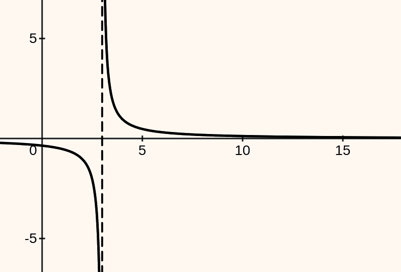
As you can see, we have a vertical asymptote at $x = 3$. In particular, we notice that when we approach the function from the left, it decreases to the bottom (that is, $-\infty$), while when we approach it from the right, it rises to $+\infty$. We want to prove this analytically:
$$ \lim_{x \to 3-} \frac{1}{x - 3} = \frac{1}{0^-} = -\infty $$
While, from the right:
$$ \lim_{x \to 3+} \frac{1}{x - 3} = \frac{1}{0^+} = +\infty $$
Exactly what we expected! Let’s now consider the following piecewise function:
$$ f(x) = \begin{cases} x^2 & x < 0\\ -\frac{1}{x} & x > 0 \end{cases} $$
Its plot is:
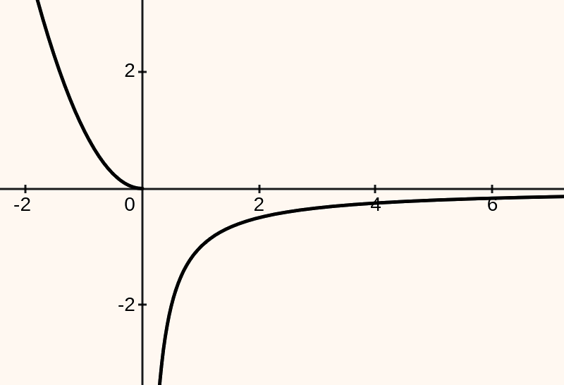
Let’s analyze its behavior as it approaches the point $x = 0$: from the left, it seems to converge to zero, while from the right it decreases to the bottom ($-\infty$). Let’s prove this analytically.
From the left, we tend to a value that is slightly less than zero, therefore we evaluate $x^2$, obtaining: $$ \lim_{x \to 0^-} f(x) = (0^-)^2 = 0 $$
While from the right, we tend to a value that is slightly more than zero, therefore we evaluate $-\frac{1}{x}$, obtaining: $$ \lim_{x \to 0^+} f(x) = \lim_{x \to 0^+} - \frac{1}{0^+} = - \infty $$
As expected. Lastly, let’s consider the function:
$$ f(x) = 2x^3 -1 $$
and let’s try to evaluate the limit at the point $x=-1$. If you take a look at its plot:
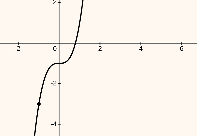
You can immediately notice that from both the left and the right, the limit of $x$ that tends to $-1$ converges to $-3$. In fact, from the left we obtain:
$$ \begin{aligned} \lim_{x \to -1^-} (2x^3 -1) &= 2(-1^-)^3 - 1\\ &= 2(-1) -1 = -2 -1\\ &= -3 \end{aligned} $$
And from the right:
$$ \begin{aligned} \lim_{x \to -1^+} (2x^3 -1) &= 2(-1^+)^3 - 1\\ &= 2(-1) -1 = -2 -1\\ &= -3 \end{aligned} $$
Therefore: $$ \lim_{x \to -1^-} f(x) = \lim_{x \to -1^+} f(x) = -3 $$
This last result allows us to state the following fundamental fact:
Given a function $$ f : A \subseteq \mathbb{R} \to \mathbb{R} $$ and an accumulation point $x_0$ for $A$, the limit $\lim_{x \to x_0} f(x) = L$ exists and it converges to $L \in \mathbb{R}$ if and only if: $$ \lim_{x \to x_0^-} f(x) = \lim_{x \to x_0^+} f(x) = L $$