Double Integrals
The theory of Riemann-integration that we have studied on the previous sections can naturally be extended by considering subsets of $\mathbb{R}^n$ with $n \geq 2$. In this lesson, we will focus on the double integral of bounded real-valued functions defined over a rectangle. As we will see later, the same ideas extend to triple integrals and to higher dimensions as well.
Let’s start by defining a rectangle:
$$ Q = [ a, b ] \times [ c, d ] $$
Let $D_1$ and $D_2$ be the partitions of $[a,b]$ and $[c,d]$, respectively:
$$ \begin{aligned} D_1 &= \left\{ a = x_0, x_1, \dots, x_{r-1}, x_r = b \right\},\\ D_2 &= \left\{ c = y_0, y_1, \dots, y_{s-1}, y_s = d \right\} \end{aligned} $$
Their product, $D = D_1 \times D_2$ is a rectangular grid partition of $Q$. Now, let’s define the intervals and their increments by:
$$ \begin{aligned} I_k &= [x_{k-1}, x_k ], \, \Delta x_k = x_k - x_{k-1}, \, k = 1, \ldots, r\\ J_h &= [y_{h-1}, y_h ], \, \Delta y_h = y_h - y_{h-1}, \, h = 1, \ldots, s \end{aligned} $$
The subrectangles of the partition are $R_{kh}=I_k\times J_h$. We can now consider a bounded real-valued function defined on the rectangle $Q$: $$ f : Q \to \mathbb{R} $$
such that: $$ m \leq f(x,y) \leq M, \quad \forall (x,y) \in Q $$
For each subrectangle $R_{kh}$, we can define:
$$ m_{kh} = \inf\limits_{(x,y) \in R_{kh}} f(x,y), \quad M_{kh} = \sup \limits_{(x,y) \in R_{kh}} f(x,y), $$
Just like for the single dimension case, we can define the lower Riemann sum:
$$ s(D, f) = \sum_{k=1}^r \sum_{n=1}^s m_{kh} \Delta x_k \Delta y_h $$
and the upper Riemann sum:
$$ S(D, f) = \sum_{k=1}^r \sum_{n=1}^s M_{kh} \Delta x_k \Delta y_h $$
Since $f$ is bounded by definition, for every partition $D$ of $Q$:
$$ m(b-a)(d-c) \leq s(D,f) \leq S(D, f) \leq M(b-a)(d-c) $$
Consequently, the supremum of all lower sums and the infimum of all upper sums exist and are finite:
$$ \inf\limits_D S(D, f), \quad \sup\limits_D s(D, f) $$
Moreover, the lower value never exceeds the upper one. We can therefore make the following definition:
A bounded function $f : Q \to \mathbb{R}$ is Riemann-integrable if:
$$ \sup\limits_D s(D, f) = \inf\limits_D S(D, f) $$ In that case, we write: $$ \iint_Q f(x) \, dx \, dy, \quad \mathcal{I}(f) $$
From a geometrical standpoint, if $f\geq 0$, the integral $\iint_q f$ represents the volume of the cylindroid lying above the rectangle $Q$ and below the grapho $z = f(x,y)$. In particular, when $f(x, y) = 1$, the double integral gives the area of $Q$.
Riemann’s Integrability Criterion
As in the one-dimensional case, we can use a criterion to determine whether a bounded function is Riemann-integrable.
Let $f: Q \to \mathbb{R}$ be a bounded function. Then $f$ is Riemann-integrable if and only if, $\forall \epsilon > 0$, $\exists D_{\epsilon} \in Q$ such that: $$ S(D_{\epsilon}, f) - s(D_{\epsilon}, f) < \epsilon $$
Once again, this criterion leads to a limit-based interpretation of the integral, let’s develop it further. We can begin by defining the concept of mesh.
Let $D = D_1 \times D_2$ a partition of $Q = [a,b] \times [c,d]$, the mesh (or norm) of $D$ is the value defined by: $$ || D || = \max \left\{ ||D_1||, \, ||D_2|| \right\} $$ where: $$ ||D_1|| = \max\limits_{1 \leq k \leq r} \Delta x_k, \quad ||D_2|| = \max\limits_{1 \leq h \leq s} \Delta y_h $$ are the meshes of $[a,b]$ and $[c,d]$, respectively.
We can now generalize the notion of a Riemann sum by choosing one value $\mu_{kh}$ for each subrectangle and defining:
$$ \sigma(D, f) = \sum_{k=1}^r \sum_{h=1}^s \mu_{kh} \Delta x_k \Delta y_h $$
where $\mu_{kh}$ is chosen such that:
$$ m_{kh} \leq u_{kh} \leq M_{kh} $$
For example, we may choose $\mu_{kh}=f(\xi_{kh},\eta_{kh})$ for some point $(\xi_{kh},\eta_{kh})\in R_{kh}$. Consequently, we can give the following definition:
The value $\ell \in \mathbb{R}$ corresponds to the limit $\sigma(D, f)$ as $|| D || \to 0$, that is: $$ \lim_{||D|| \to 0} \sigma(D, f) = \ell $$ If, $\forall \epsilon > 0, \exists \delta_{\epsilon} > 0$ such that:
$$ \left\vert \sigma(D, f) - l \right\vert < \epsilon $$ for every partition $D$ of $Q$ with $||D|| < \delta_{\epsilon}$ and every choice of the values $\mu_{kh}$ satisfying $m_{kh}\leq\mu_{kh}\leq M_{kh}$.
This gives an equivalent definition of the double Riemann integral:
Let $f : Q \to \mathbb{R}$ be a bounded function on the rectangle $Q$. Then, $f$ is Riemann-integrable if and only if: $$ \lim_{||D|| \to 0} \sigma (D, f) = \ell \in \mathbb{R} $$ In that case, we write:
$$ \iint_Q f(x, y) \, dx \, dy = \lim_{||D || \to 0} \sigma (D, f) $$
Iterated Integrals
Let’s now look at a practical technique for evaluating double integrals, known as reduction to iterated integrals.
Let $f$ be a Riemann-integrable function on $Q = [a,b]\times [c,d]$. If, $\forall y\in[c,d]$, the function $x\mapsto f(x,y)$ is Riemann-integrable on $[a,b]$, we can define: $$ G(y) = \int_a^b f(x, y) \, dx $$ Then $G$ is Riemann-integrable on $[c,d]$, and:
$$ \iint_Q f (x) \, dx \, dy = \int_c^d G(y) \, dy = \int_c^d \left(\int_a^b f(x, y) \, dx \right) dy $$
Similarly, if, for every $x\in[a,b]$, the function $y\mapsto f(x,y)$ is Riemann-integrable on $[c,d]$, we define:
$$ H(x) = \int_c^d f(x,y) \, dy $$
Then $H$ is Riemann-integrable on $[a,b]$, and:
$$ \iint_Q f (x) \, dx \, dy = \int_a^b H(x) \, dx = \int_a^b \left(\int_c^d f(x, y) \, dy \right) dx $$
Let’s look at an example. We want to evaluate the following double integral:
$$ I = \iint_Q (x + y) \, dx \, dy $$
Where:
$$ Q = \left\{ (x, y) \in \mathbb{R}^2 : 0 \leq x \leq 1, \, 0 \leq y \leq 2 \right\} $$
We notice that the domain is the rectangle $Q=[0,1]\times[0,2]$, and the function $f(x,y)=x+y$ is continuous on $Q$. We can therefore evaluate the double integral as an iterated integral:
$$ \begin{aligned} I &= \int_0^1 \left( \int_0^2 (x + y) \, dy \right) \, dx\\ &= \int_0^1 \left[ xy + \frac{y^2}{2} \right]_0^2 \, dx\\ &= \int_0^1 (2x + 2) \, dx\\ &= \left[ x^2 + 2x \right]_0^1\\ &= 1 + 2\\ &= \boxed{3} \end{aligned} $$
If we reverse the order of integration, we obtain the same result:
$$ \begin{aligned} I &= \int_0^2 \left( \int_0^1 (x + y) \, dx \right) \, dy\\ &= \int_0^2 \left[ \frac{x^2}{2} + xy \right]_0^1 \, dy\\ &= \int_0^2 \left( \frac{1}{2} + y \right) \, dy\\ &= \left[ \frac{y}{2} + \frac{y^2}{2} \right]_0^2\\ &= 1 + 2\\ &= \boxed{3} \end{aligned} $$
Let’s now look at the following example:
$$ \iint_Q \frac{1}{x} \, dx \, dy, \quad Q = [0,1] \times [0,1] $$
Just like before, $Q$ still represents a rectangle. However, the function $f(x,y)=1/x$ is unbounded near $x=0$ and is not defined there Therefore, it does not satisfy the hypotheses of the proper double Riemann integral we have defined above. Still, we can examine the corresponding improper double integral by truncating the domain away from $x=0$:
$$ \begin{aligned} I_\epsilon &=\int_0^1\left(\int_\epsilon^1\frac{1}{x}\,dx\right) \, dy\\ &=\int_0^1[-\log\epsilon] \,dy\\ &=-\log\epsilon. \end{aligned} $$
Thus the improper double integral diverges:
$$ \lim_{\epsilon\to 0^+}I_{\epsilon} =\lim_{\epsilon\to 0^+}(-\log\epsilon) =+\infty, $$
Theory of Measure
Although the theory we have introduced so far allows us to determine the area of a given rectangle $Q = [a,b] \times [c,d]$, it does not yet provide a systematic way to assign an area to more general subsets of $\mathbb{R}^2$ such as triangles, discs or, more generally, any other bounded regions. To address this issue, we need to introduce a more refined theory of measure.
Let’s begin with a bounded set $\Omega\subseteq\mathbb{R}^2$ contained in a rectangle $Q$ and let’s divide $Q$ into a finite number of smaller rectangles, say:
$$ Q_1, Q_2, \ldots, Q_n $$
Then, let’s associate an area $|Q_i|$ with each rectangle. Relative to $\Omega$, each rectangle falls into one of three cases:
- The rectangle is completely contained into $\Omega$;
- The rectangle is disjoint from $\Omega$;
- The rectangle intersects $\Omega$ but is not completely contained in it; in particular, it meets the boundary of $\Omega$.
In the first two cases, we know whether the entire rectangle belongs to the set. In the third case, we must use an approximation to determine how much of the rectangle belongs to $\Omega$.
If we now recall that an elementary set is a finite union of rectangles whose interiors are pairwise disjoint, its area, denoted by $m(A)$, is the sum of the areas of those rectangles, we can therefore define the internal Peano–Jordan measure of $\Omega$ by
$$ m_i(\Omega) = \sup\limits_{A \subseteq \Omega} m(A) $$
In other words, $A$ ranges over all elementary sets contained in $\Omega$. We use a supremum because an elementary set of greatest area may not exist; the supremum is the least upper bound of the areas of all such sets.
Similarly, we define the external Peano-Jordan measure of $\Omega$ as:
$$ m_e(\Omega) = \inf\limits_{B \supseteq \Omega} m(B) $$
Here, $B$ ranges over all elementary sets containing $\Omega$. We can therefore make the following definition:
A bounded subset $\Omega \subseteq \mathbb{R}^2$ is Peano-Jordan measurable if: $$ m(\Omega) = m_i(\Omega) = m_e (\Omega) $$ Their common value is called the Peano–Jordan measure of $\Omega$ and is denoted by $m(\Omega)$.
Let’s now apply this theory of measure to the Riemann integral. We begin by defining the characteristic function of $\Omega$:
$$ \chi_{\Omega}(x,y) = \begin{cases} 1 \iff (x, y) \in \Omega\\ 0 \iff (x, y) \notin \Omega \end{cases} $$
This function turns a geometrical problem into an analytical one. Let’s now consider a subrectangle $Q_i$ of a partition of the containing rectangle $Q$. There are three possibilities:
- The rectangle is contained in $\Omega$: he characteristic function is identically equal to $1$ on $Q_i$ and therefore: $$ \inf\limits_{Q_i} \chi_{\Omega} = \sup\limits_{Q_i} \chi_{\Omega} = 1 $$
- The rectangle is disjoint from $\Omega$: the characteristic function identically equal to $0$ on $Q_i$ and therefore:
$$ \inf\limits_{Q_i} \chi_{\Omega} = \sup\limits_{Q_i} \chi_{\Omega} = 0 $$ 3. The rectangle intersects $\Omega$ but is not contained in it: the characteristic function takes both values $0$ and $1$ on $Q_i$ and therefore: $$ \inf\limits_{Q_i} \chi_{\Omega} = 0, \quad \sup\limits_{Q_i} \chi_{\Omega} = 1 $$
In the third case, the lower sum contributes $0$, while the upper sum contributes the full area $|Q_i|$. Thus, the lower and upper sums for $\chi_\Omega$ can be written as
$$ s(D, \chi_{\Omega}) = \sum_{Q_i \subseteq \Omega} | Q_i |, \quad S(D, \chi_{\Omega}) = \sum_{Q_i \cap \Omega \neq \emptyset} |Q_i| $$
Their difference is exactly the total area of the subrectangles on which $\chi_\Omega$ takes both values $0$ and $1$ (the subrectangles that meet the boundary of $\Omega$). In other words:
$$ S(D,\chi_\Omega)-s(D,\chi_\Omega) = \sum_{\substack{Q_i\cap\Omega\neq\varnothing\\Q_i\nsubseteq\Omega}}|Q_i| $$
If we now apply the Riemann’s integrability criterion, we obtain:
$$ \chi_{\Omega} \in \mathcal{R}(\Omega) \iff \forall \epsilon > 0, \exists D_{\epsilon} : S(D_{\epsilon}, \chi_{\Omega}) - s(D_{\epsilon}, \chi_{\Omega}) < \epsilon $$
But since this difference is the total area of the boundary-intersecting subrectangles, we obtain the following characterization:
A bounded subset $\Omega \subseteq \mathbb{R}^2$ is P-J measurable if and only if $\chi_{\Omega} \in \mathcal{R}(Q)$; that is, if its characteristic function is Riemann-integrable on a rectangle $Q$ containing $\Omega$. In that case, we write: $$ m(\Omega) = \iint_Q \chi_{\Omega}(x,y) \, dx \, dy $$
Another useful characterization involves the concept of measure zero.
A bounded subset $\Omega \subseteq \mathbb{R}^2$ has Jordan measure zero if $\forall \epsilon > 0$, there exists a finite collection of rectangles $R_1, \ldots, R_{N_{\epsilon}}$ that covers $\Omega$ and whose total area is less than $\epsilon$. In other words: $$ \Omega \subseteq \bigcup_{i=1}^{N_{\epsilon}} R_i, \quad \sum_{i=1}^{N_{\epsilon}} |R_i| < \epsilon $$
The crucial point is that a Jordan null set must be coverable by finitely many rectangles. If we instead allow a countable collection of rectangles, we obtain the definition of Lebesgue null set:
A subset $\Omega \subseteq \mathbb{R}^2$ has Lebesgue measure zero if, $\forall \epsilon > 0$, there exists a countable collection of rectangles $R_1, R_2, \ldots$ that covers $\Omega$ and whose total are is less than $\epsilon$. In other words: $$ \Omega \subseteq \bigcup_{i=1}^{\infty} R_i, \quad \sum_{i=1}^{\infty} |R_i| < \epsilon $$
Consequently, every Jordan null set is also Lebesgue null but the converse is not generally true. For example, the set of points $[0, 1]^2$ with two rational coordinates is countable and hence Lebesgue null, but since it is dense in the square and thus not Jordan null.
With this theoretical foundation, we can state the following important integrability criterion, know as Lebesgue’s criterion for Riemann integrability:
Let $Q$ be a rectangle and let $f : Q \to \mathbb{R}$ be a bounded function. Then, $f$ is Riemann-integrable if and only if the set of points at which $f$ is discontinuous has Lebesgue measure zero.
Properties of the Integral
Just as in the one-dimensional case, the double integral can be viewed as a functional since it maps every function $f \in \mathcal{R}(\Omega)$ to a real number. Specifically, it is a linear functional since, given $f, g \in \mathcal{R}(\Omega)$ and $\alpha, \beta \in \mathbb{R}$ with $\alpha f + \Beta g \in \mathcal{R}(\Omega)$, we have that:
$$ \iint_{\Omega} (\alpha f + \beta g) \, dx \, dy = \alpha \iint_{\Omega} f \, dx \, dy + \beta \iint_{\Omega} g \, dx \, dy $$
Furthermore, let $\Omega_1, \Omega_2 \subseteq \mathbb{R}^2$ be two bounded P-J measurable subsets such that their intersection has Jordan measure zero. If a bounded function $f$ is Riemann integrable on each of them, then it is also Riemann integrable on their union and the following formula holds:
$$ \iint_{\Omega_1 \cup \Omega_2} f \, dx \, dy = \int_{\Omega_1} f \, dx \, dy + \iint_{\Omega_2} f \, dx \, dy $$
Finally, suppose that $\Omega$ is P-J measurable with positive area and that $f$ is a bounded and Riemann-integrable function on $\Omega$. Additionally, let’s define the following two quantities:
$$ m_f = \inf\limits_{(x, y) \in \Omega} f(x,y), \qquad M_f = \sup\limits_{(x, y) \in \Omega} f(x, y) $$
Then, we can define the average value over $\Omega$ as:
$$ f_{\text{avg}} = \frac{1}{|\Omega|} \iint_{\Omega} f(x, y) \, dx \, dy $$
where $|\Omega| = m(\Omega) > 0$ is the area of $\Omega$ which satisfied the following inequality:
$$ m_f \leq \underbrace{\frac{1}{|\Omega|} \iint_{\Omega} f(x, y) \, dx \, dy}_{\text{average value}} \leq M_f $$
Change of Variables
One of the most commonly used techniques for evaluating double integrals is to perform a change of variables in the plane. This technique does more than simply transform the expression of the function being integrated: it also changes the region over which the integration takes place. The central idea is therefore to understand how this transformation affects the region of integration and, in particular, how it changes area.
Let’s start by considering the double integral of a given function:
$$ \iint_Q f(x,y) \, dx \, dy $$
Here, $dx \, dy$ denotes the Cartesian area element. Suppose that we want to describe the same region using another pair of variables, say $u$ and $v$. We do so through a bijective transformation:
$$ t : \Omega \to Q $$
defined by:
$$ T(u,v) = \left( \varphi(u,v), \psi(u,v) \right) \iff \begin{cases} x = \varphi(u,v)\\ y = \psi(u,v) \end{cases} $$
The issue we want to address is how the area of a changes under this substitution. Let’s begin with the simplest case first: a linear transformation $T : \mathbb{R}^2 \to \mathbb{R}^2$ defined by:
$$ \begin{cases} x = au + bv\\ y = cu + dv \end{cases} \iff \begin{pmatrix} x\\ y \end{pmatrix} = \underbrace{\begin{pmatrix} a & b \\ c & d \end{pmatrix}}_{A} \begin{pmatrix} u\\ v \end{pmatrix} $$
The $A$ matrix represent this transformation. Let’s consider the unit square in the $uv$-plane, whose vertical vertices are $(0,0)$, $(1,0)$, $(0,1)$, and $(1,1)$. The transformation $T$ maps these vertices as follows:
$$ \begin{aligned} (0,0) &\longmapsto (0,0)\\ (1,0) &\longmapsto (a,c)\\ (0,1) &\longmapsto (b,d)\\ (1,1) &\longmapsto (a + b,c + d) \end{aligned} $$
The square is therefore mapped to a parallelogram generated by the two vectors $\mathbf{a}=(a,c)$ and $\mathbf{b}=(b,d)$. Geometrically, the $uv$-plane contains a square of area $1$:
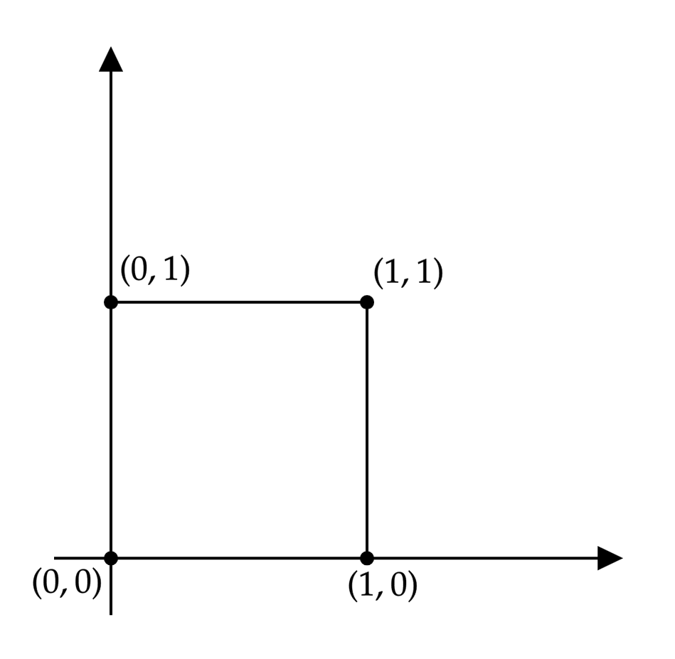
whereas its image in the $xy$-plane is the parallelogram generated by these two vectors:
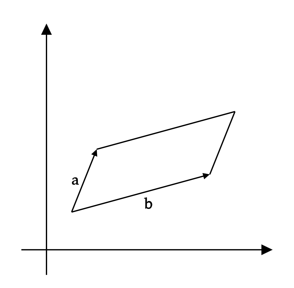
To determine the change in area, we need to calculate the are of the parallelogram using the standard formula base * height. We choose $\mathbf{a}$ as the base, its length is:
$$ || \textbf{a} || = \sqrt{a^2 + c^2} $$
The height, instead, corresponds to the magnitude of the component of $\mathbf{b}$ perpendicular to $\mathbf{a}$. The resulting area is:
$$ \text{Area}(T([0,1]^2)) = |ad - bc|. $$
This is precisely the absolute value of the determinant of $A$:
$$ \det(A) = \begin{vmatrix} a & b\\ c & d \end{vmatrix} = ad - bc $$
Since the original square has area $1$, the ratio between the area of the transformed parallelogram and the area of the original square is:
$$ |\det A| = |ad - bc | $$
If $\det A=0$, the parallelogram degenerates into a line segment and its area is zero. Otherwise, the transformation is invertible. Now let’s consider a more general rectangle in the $uv$-plane, with side lengths $\Delta u$ and $\Delta v$. Its area is:
$$ \Delta A_{uv} = \Delta u , \Delta v. $$
Under the linear transformation, its sides are mapped to vectors proportional to the columns of $A$, scaled by $\Delta u$ and $\Delta v$, respectively. The resulting parallelogram therefore has area equal to:
$$ \Delta A_{xy} = |ad - bc | \Delta u \Delta v $$
Or, equivalently:
$$ \Delta A_{xy} = |ad - bc | \Delta A_{uv} $$
We conclude that, under a linear transformation, the absolute value of the determinant is the factor by which areas are multiplied.
Let’s now consider an affine transformation defined by:
$$ T(u,v) = A \begin{pmatrix} u\\ v \end{pmatrix} + \begin{pmatrix} h\\ k \end{pmatrix} $$
That is:
$$ \begin{cases} x = au + bv + h\\ y = cu + dv + k \end{cases} $$
In addition to the linear transformation represented by $A$, we now have a translation by the vector $(h,k)$, which moves every point by the same vector and therefore leaves lengths, angles and areas unchanged. Consequently, the area formula is the same as in the linear case:
$$ \Delta A_{xy} = | ad - bc | \Delta u \Delta v = | ad - bc | \Delta A_{uv} $$
In other words, the translation has no effect on the area factor. Only the linear part of the affine transformation matters. However, a general transformation is rarely affine as it typically exhibits curvature, curvature, deformation or other distortions across the domain. We therefore need a way to reduce it to the linear case, at least locally.
Let’s consider a general transformation of the form:
$$ T(u,v) = \left( \varphi(u,v), \psi(u,v) \right) \iff \begin{cases} x = \varphi(u,v)\\ y = \psi(u,v) \end{cases} $$
Suppose that $\varphi$ and $\psi$ are differentiable. In this case, there is generally no single scaling factor that is valid throughout the entire domain. The key idea is therefore to consider a sufficiently small neighborhood of a point and observe how a differentiable transformation behaves, to first order, like its tangent linear transformation.
Let’s choose a point $P=(u_0, v_0)$ and consider the following two increments:
$$ \Delta u = u - u_0, \quad \Delta v = v - v_0 $$
By differentiability, we obtain:
$$ \begin{aligned} \Delta x &= \varphi \left( u_0 + \Delta u, v_0 + \Delta v \right) - \varphi(u_0, v_0)\\ &= \frac{\partial \varphi}{\partial u}(P) \Delta u + \frac{\partial \varphi}{\partial v}(P) \Delta v + o(\rho) \end{aligned} $$
Where:
$$ \rho = \sqrt{ \left( \Delta u \right)^2 + \left( \Delta v \right)^2} $$
and $o(\rho)$ denotes a remainder whose ratio to $\rho$ tends to zero as $\rho\to0$. Likewise:
$$ \Delta y = \frac{\partial \psi}{\partial u}(P) \Delta u + \frac{\partial \psi}{\partial v}(P) \Delta v + o(\rho) $$
If we neglect the error terms, we obtain the following linear approximation:
$$ \begin{aligned} \Delta x &\approx \varphi_u(P) \Delta u + \varphi_v (P) \Delta v\\ \Delta y &\approx \psi_u(P) \Delta u + \psi_v (P) \Delta v \end{aligned} $$
In matrix notation:
$$ \begin{pmatrix} \Delta x\\ \Delta y \end{pmatrix} \approx \underbrace{\begin{pmatrix} \varphi_u(P) & \varphi_v(P)\\[0.4em] \psi_u(P) & \psi_v (P)\end{pmatrix}}_{DT(P)} \cdot \begin{pmatrix} \Delta u\\ \Delta v \end{pmatrix} $$
The matrix $DT(P)$ is the Jacobian matrix of the transformation at $P$. It is used to describe to the first order how the image of a point changes when the original point undergoes a small displacement. Its columns are the tangent vectors to the image curves obtained by varying $u$ and $v$, respectively.
Applying the formula for the area of the parallelogram to this linear approximation, we obtain:
$$ \Delta A_{xy} \approx | \det(DT(P)) | \Delta u \Delta v $$
The determinant is:
$$ \det(DT(P)) = \begin{vmatrix} \varphi_u(P) & \varphi_v(P)\\[0.4em] \psi_u(P) & \psi_v(P) \end{vmatrix} = \varphi_u (P) \psi_v(P) - \varphi_v(P) \psi_u (P) $$
We can therefore define the Jacobian determinant of the transformation by:
$$ J_T(u,v) = \frac{\partial(\varphi, \psi)}{\partial(u,v)} = \begin{vmatrix} \varphi_u & \varphi_v\\ \psi_u & \psi_v \end{vmatrix} $$
Its absolute value measures the local scaling factor for areas.
We now have the ingredients needed to state the change of variables formula for a double integral. A standard version of the theorem is the following.
Let $U, V \subseteq \mathbb{R}^2$ be open sets and suppose that $T : U \to V$ is a $C^1$ diffeomorphism. Let $\Omega \subset U$ be a bounded P-J measurable region and set $Q = T(\Omega)$. If $f$ is Riemann-integrable on $Q$, then: $$ \iint_Q f(x,y) \, dx \, dy = \iint_{\Omega} f(\varphi(u,v), \psi(u,v)) |J_T(u,v)| \, du \, dv $$ Where a $C^1$ diffeomorphism is a bijective, continuously differentiable transformation with a continuously differentiable inverse. In particular, its Jacobian determinant is nonzero.
The formula can be understood intuitively through Riemann sums as follows. Let’s divide the parameter region $\Omega$ into small rectangles $R_i$, each with area equal to:
$$ \Delta A_i = \Delta u_i \Delta v_i $$
Then, choose a sample point $(u_i, v_i) \in R_i$. For sufficiently small rectangles, the area of the image region is approximately:
$$ \Delta A'_i \approx | J_T(u_i, v_i)| \Delta u_i \Delta v_i $$
The contribution of this image region to the integral is therefore approximately:
$$ f(T(u_i, v_i)) |J_T(u_i, v_i)| \Delta u_i \Delta v_i $$
Summing these contributions gives:
$$ \sum_i f(T(u_i, v_i)) |J_T(u_i, v_i)| \Delta u_i \Delta v_i $$
We notice that this is exactly a Riemann sum on the parameter region $\Omega$ relative to the function:
$$ g(u,v) = f(\varphi(u,v), \psi(u,v)) |J_T(u,v)| $$
As the mesh of the partition tends to zero, these sums converge to the integral of $g$ over $\Omega$, which gives the change of variable formula of the previous theorem.
Polar Coordinates
A particularly important case of the previous change of variable formula is the conversion to polar coordinates. This technique is especially useful when the domain of the integration or the integrand involves a circle, a disk or an expression of the form $x^2 + y^2$.
In polar coordinates, the transformation becomes:
$$ \begin{cases} x = r \cos \theta\\ y = r \sin \theta \end{cases} $$
where $r$ denotes the distance from the origin and $\theta$ is the angle that the segment from the origin to the point makes with the positive $x$-axis. Graphically, this is:
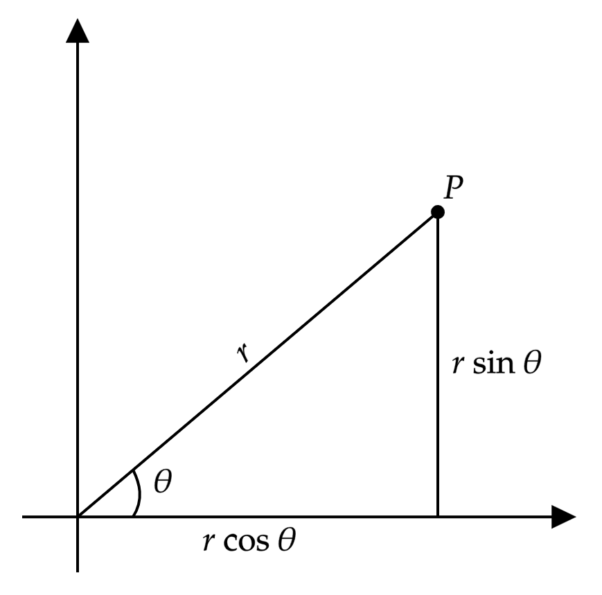
The transformation can simplify many expressions. For example:
$$ x^2 + y^2 = r^2 \cos^2 \theta + r^2 \sin^2 \theta = r^2 $$
Which implies that
$$ r = \sqrt{x^2 + y^2} $$
Let’s calculate the Jacobian determinant for this substitution. The Jacobian matrix is formed by the following partial derivatives:
$$ J(r, \theta) = \begin{vmatrix} \dfrac{\partial x}{\partial r} & \dfrac{\partial x}{\partial \theta}\\[1.2em] \dfrac{\partial y}{\partial r} & \dfrac{\partial y}{\partial \theta}\\ \end{vmatrix} $$
Evaluating these derivatives gives:
$$ \begin{aligned} x_r &= \cos \theta, \quad y_{\theta} = -r \sin \theta\\ y_r &= \sin \theta, \quad y_{\theta} = r \cos \theta \end{aligned} $$
Which corresponds to:
$$ \begin{aligned} J(r, \theta) &= \begin{vmatrix} \cos \theta & -r \sin \theta\\ \sin \theta & r \cos \theta \end{vmatrix}\\[0.5em] &= r \cos^2 \theta + r \sin^2 \theta\\ &= r (\cos^2 + \sin^2 \theta)\\ &= r \end{aligned} $$
Since $r \geq 0$, the absolute value of the Jacobian determinant is also $r$. Thus, the Cartesian area element transforms according to the following area element:
$$ dx \, dy = r \, dr \, d\theta $$
This is a shorthand notation for the scale relationship of the area given by the Jacobian. The double integral formula becomes:
$$ \iint_Q f(x,y) \, dx \, dy = \iint_{\Omega} f(r \cos \theta, r \sin \theta) \, r \, dr \, d \theta $$
where $\Omega$ is the region in the $(r, \theta)$-plane corresponding to $Q$. We notice that the polar coordinate map is not one-to-one at the origin since the angle is undefined there. However, this causes no difficulty for integration as the origin is a set of area zero. Angular boundary rays can likewise be handled as boundary sets of area zero.
Let’s conclude this lesson with a practical example. We want to evaluate:
$$ \iint_Q \sqrt{x^2 + y^2} \, dx \, dy $$
Where:
$$ Q = \left\{ (x, y) \in \mathbb{R}^2 : x^2 + y^2 \leq 4x \right\} $$
Let’s first analyze the domain:
$$ x^2 + y^2 \leq 4x \iff x^2 - 4x + y^2 \leq 0 $$
Let’s express this by completing the square.
From the identity $(a-b)^2 = a^2 - 2ab + b^2$ we notice that:
$$ a = x \implies -2xb = -4x \iff b = 2 $$
Therefore, $-2ab = -4x$ and thus $(x-2)^2 = x^2- 4x + 4$. In our example, this corresponds to $x^2 - 4x = (x-2)^2 - 4$. By comparing this with the standard equation of a disk:
$$ (x-a)^2 + (y-b)^2 \leq R^2 $$
we recognize a disk centered at $C=(a,b)=(2,0)$ with radius $R=2$. Now let’s switch to polar coordinates. We first need to determine the new limits of integration. Substituting:
$$ x = r \cos \theta, \quad y = r \sin \theta $$
into the inequality defining $Q$, we obtain:
$$ r^2 \cos^2 \theta + r^2 \sin^2 \theta \leq 4r \cos \theta $$
Then, by using the trigonometric identity $\cos^2\theta+\sin^2\theta=1$, we get:
$$ r^2 \leq 4r \cos \theta $$
Since $r \geq 0$, the origin is included and for $r>0$ we can divide by $r$ to obtain:
$$ 0 \leq r \leq 4 \cos \theta $$
For the upper bound to be nonnegative, we need $\cos\theta \geq 0$. We can therefore choose:
$$ - \frac{\pi}{2} \leq \theta \leq \frac{\pi}{2} $$
Including the origin, the domain in polar coordinates is therefore described by:
$$ - \frac{\pi}{2} \leq \theta \leq \frac{\pi}{2}, \quad 0 \leq r \leq 4 \cos \theta $$
We can now transform the integrand. Since $r= \sqrt{x^2+y^2}$, we have:
$$ f(r \cos \theta, r \sin \theta) = r $$
The Jacobian contributes the factor $r$, so the integrand together with the area element becomes:
$$ \sqrt{x^2 + y^2} \, dx \, dy \longmapsto r \cdot r \, dr \, d \theta = r^2 \, dr \, d\theta $$
The new integral is therefore:
$$ \int_{-\pi/2}^{\pi/2} \int_0^{4 \cos \theta} r^2 \, dr \, d\theta $$
We can now evaluate it as an iterated integral:
$$ \begin{aligned} \int_{-\pi/2}^{\pi/2} \left( \int_0^{4 \cos \theta} r^2 \, dr \right) \, d\theta &= \int_{-\pi/2}^{\pi/2} \left[ \frac{r^3}{3} \right]_0^{4 \cos \theta} \, d\theta\\ &= \int_{-\pi/2}^{\pi/2} \frac{64}{3} \cos^3 \theta \, d\theta\\ &= \frac{64}{3} \int_{-\pi/2}^{\pi/2}\cos^3 \theta \, d\theta \end{aligned} $$
Since $\cos^3 \theta$ is an even function, we can write:
$$ \frac{64}{3} \int_{-\pi/2}^{\pi/2}\cos^3 \theta \, d\theta = \frac{128}{3} \int_0^{\pi/2} \cos^3 \theta \, d\theta $$
To evaluate the remaining integral, we rewrite:
$$ cos^3 \theta = \cos \theta (1 - \sin^2 \theta) $$
and use the substitution $t = \sin \theta$ so that $dt = \cos \theta \, d \theta$. The limits of integration change from $\theta = 0$ and $\theta = \frac{\pi}{2}$ to $t = 0$ and $t = 1$, respectively. Therefore, we conclude that:
$$ \begin{aligned} \frac{128}{3} \int_0^{\pi/2} \cos^3 \theta \, d\theta &= \frac{128}{3} \int_0^1 (1 - t^2) \, dt\\ &= \frac{128}{3} \left[t - \frac{t^3}{3} \right]_0^1\\ &= \frac{128}{3} \cdot \frac{2}{3}\\[0.5em] &= \frac{256}{9}\\ &\approx \boxed{28.44} \end{aligned} $$