Riemann Integral
To calculate the area of common geometric figures (such as a triangle or a square), we use formulas derived from Euclidean geometry. If, however, the geometric shape to be measured is represented by an arbitrary curve, traditional formulas are no longer suitable. The Riemann integral addresses this limitation by approximating the are under a curve using a sum of rectangles, that is, by adding up the areas of small portions of the curve using the usual “base * height” formula.
As a first example, let’s consider the function $f(x) = x^2$ and let’s set the goal of calculating the area enclosed between the $x$-axis, the $f(x)$ graph on the interval $[0,b]$ and the two vertical boundaries $x=0$ and $x=b$. In other words:
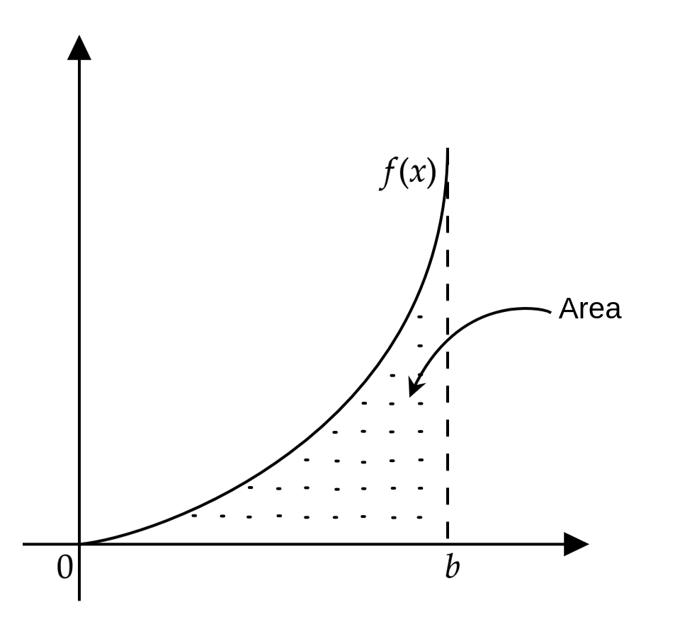
Let’s begin by dividing the $[0, b]$ interval in $n$ distinct subintervals $[x_{i-1}, x_i]$ with a width equal to $\frac{b}{n}$. That is:
$$ x_0 = 0, \ \ x_1 = \frac{b}{n}, \ \ x_2 = \frac{2b}{n}, \ \ \ldots \ \ x_i = \frac{i}{n} b, \ \ \ldots \ \ x_n = b $$
By doing this, we will obtain a region formed by the union of rectangles, each having as a base the interval $[x_{i-1}, x_i]$, a width $\frac{b}{n}$ and a height of $f(x_{i-1}) = x^2_{i-1}$. Graphically:
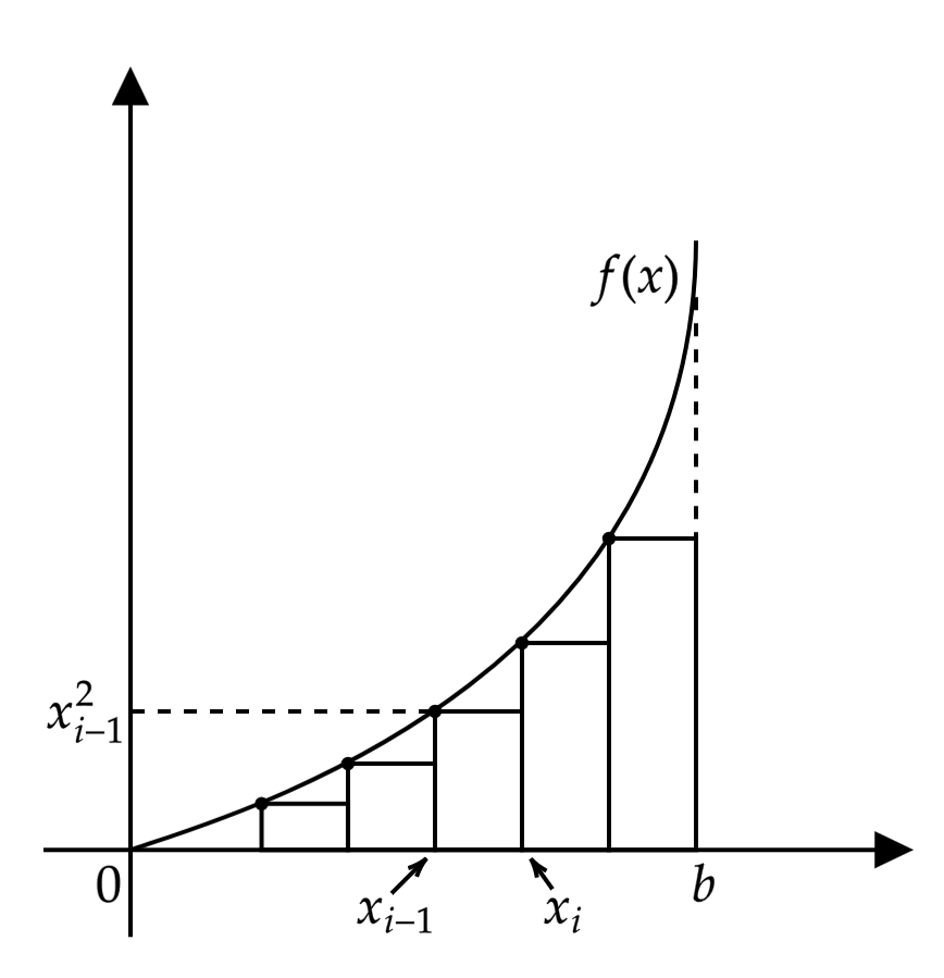
Therefore, the total area is given by the sum of the areas of the rectangles, that is:
$$ \begin{aligned} A_f &= f(x_0)(x_1 - x_0) + f(x_1)(x_2 - x_1) + \dots + f(x_{n-1})(x_n - x_{n-1})\\ &= \sum_{i=1}^{n} \underbrace{f(x_{i-1})}_{\text{height}} \cdot \underbrace{(x_i - x_{i-1})}_{\text{base}}\\ &= \sum_{i=1}^n x^2_{i-1} \cdot \frac{b}{n} = \boxed{\frac{b}{n} \sum_{i=1}^n x^2_{i-1}} \end{aligned} $$
We notice that this sum provides a lower approximation of the area. Let’s now consider the region formed by the union of rectangles with the same base and width, but with a height given by $f(x_i) = x^2_i$.
Graphically, this corresponds to:
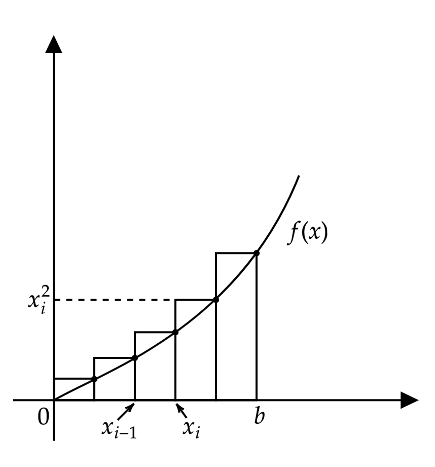
In this case, the area is:
$$ A_f = \sum_{i=1}^n f(x_i) (x_i - x_{i-1}) = \boxed{ \frac{b}{n} \sum_{i=1}^n x^2_i} $$
This time, however, the sum provides a higher approximation of the area. Therefore, we have:
$$ \underbrace{\frac{b}{n} \sum_{i=1}^n x^2_{i-1}}_{\text{Lower Sum}} < A_f < \underbrace{\frac{b}{n} \sum_{i=1}^n x^2_i}_{\text{Upper Sum}} $$
Definition
Let’s now try to formalize this procedure; by doing so, we will naturally arrive to the definition of the Riemann integral.
Let $[a, b]$ be an interval. A partition $D$ of $[a, b]$ is an ordered set formed by the $n+1$ distinct points of the interval such that:
$$ a = x_0 < x_1 < \dots < x_{n-1} < x_n = b $$
Moreover, let $f : [a, b] \to \mathbb{R}$ be a bounded function on $[a, b]$. Then, by definition, this means that:
$$ \exists m, M \ : \ m \leq f(x) \leq M \qquad \forall x \in [a, b] $$
Additionally, let $D = \{ x_0, \ldots, x_n \}$ a partition of $[a, b]$; then, the $n+1$ points identify $n$ intervals $[x_{i-1}, x_i]$ with $i=1, 2, \ldots, n$. Therefore, we have:
$$ m_i = \inf \left\{ \ f(x) : x \in [x_{i-1}, x_i] \ \right\}, $$
$$ M_i = \sup \left\{ \ f(x) : x \in [x_{i-1}, x_i] \ \right\} $$
By setting $\Delta x_i = x_i - x_{i-1}$, we can define the following two integral sums:
$$ s(D, f) = \sum_{i=1}^n m_i \cdot \Delta x_i $$
$$ S(D, f) = \sum_{i=1}^n M_i \cdot \Delta x_i $$
Where $s(D, f)$ is called the lower Riemann sum and $S(D, f)$ the upper Riemann sum. Additionally, since $f$ is bounded by definition, for every partition $D$ of $[a, b]$ we have that:
$$ m(b-a) \leq s(D, f) \leq S(D, f) \leq M(b - a) $$
Thus, the following two values exist and are finite:
$$ \inf S(D, f), \ \ \sup s(D, f) $$
These are the infimum of the upper Riemann sum and the supremum of the lower Riemann sum, respectively. When these two quantities are equal, the function is integrable. More formally:
A bounded function $f : [a, b] \to \mathbb{R}$ is Riemann integrable if: $$ \sup s(D, f) = \inf S(D, f) $$ In that case, we write: $$ \int_a^b f(x) \, dx, \quad \mathcal{I}(f) $$
Riemann’s Integrability Criterion
Once we have defined the notion of the Riemann integral, we need to characterize it; that is, find a criterion to determine when a given function is integrable. In order to do this, we can prove the following theorem.
A bounded function $f : [a, b] \to \mathbb{R}$ is Riemann integrable if and only if, $\forall \epsilon > 0$, there exists a partition $D_{\epsilon}$ of $[a, b]$ such that ($\clubsuit$): $$ S(D_{\epsilon}, f) - s(D_{\epsilon}, f) < \epsilon $$
Let’s assume that $\clubsuit$ holds, then:
$$ 0 \leq \inf S - \sup s \leq S(D_{\epsilon}, f) - s(D_{\epsilon}, f) < \epsilon $$
Therefore, we have that $\inf S = \sup s$ and thus $f$ is Riemann integrable. Likewise, if $f$ is Riemann integrable, then given an $\epsilon$, there exists a partition $D_1$ such that:
$$ \mathcal{I}(f) - s(D_1, f) < \frac{1}{2} \epsilon $$
and another partition $D_2$ such that:
$$ S(D_2, f) - \mathcal{I}(f) < \frac{1}{2} \epsilon $$
Finally, let’s introduce $D_3$ as a finer partition containing both $D_1$ and $D_2$. We obtain:
$$ S(D_3, f) - s(D_3, f) \leq S(D_2, f) - s(D_1, f) < \epsilon $$
which proves $\clubsuit$ $\blacksquare$.
This criterion allows us to view the Riemann integral as the value to which the lower and upper sums converge as the “width” of the partition of $[a, b]$ tends to zero. To formalize this concept and define the Riemann integral in terms of limits, let’s introduce the following definition:
Let $D$ be a partition of $[a, b]$, the mesh (or norm) of $D$ is the value defined by: $$ || D || = \max \{ (x_i - x_{i-1}) \} $$
Next, let’s generalize the notion of Riemann sums:
$$ \sigma(D, f) = \sum_{i=1}^n \mu_i \Delta x_i $$
where $\mu_i$ is chosen such that:
$$ m_i \leq \mu_i \leq M_i $$
Consequently, the following inequality holds:
$$ s(D, f) \leq \sigma(D, f) \leq S(D, f) $$
We can now define the following limit.
The value $l \in \mathbb{R}$ corresponds to the limit of $\sigma(D, f)$ as $|| D ||$ tends to zero, that is: $$ \lim_{||D|| \to 0} \sigma(D, f) = l $$ if, $\forall \epsilon > 0, \exists \delta_{\epsilon} > 0$ such that: $$ | \sigma(D, f) - l | < \epsilon $$ for all partitions $D$ with $|| D || < \delta_{\epsilon}$ and for all $\mu_i$.
This allows us to give the following definition of the Riemann integral.
A bounded function $f : [a, b] \to \mathbb{R}$ is Riemann integrable if and only if the following limit exists and is finite: $$ \lim_{||D|| \to 0} \sigma(D, f) $$ In that case, we write: $$ \int_a^b f(x) \, dx = \lim_{||D|| \to 0} \sigma(D, f) $$
Geometrical Interpretation
The Riemann integral has some important geometrical properties. Specifically, the lower sum $s(D,f)$ represents the area of the rectilinear polygon contained within the set $T$ defined as follows:
$$ T = \left\{ (x, y) \in \mathbb{R}^2 : a \leq x \leq b, \, 0 \leq y \leq f(x) \right\} $$
On the other hand, the upper sum $S(D, f)$ represents the area of the rectilinear polygon that contains $T$. Finally, the set $T$ represents a curvilinear trapezoid with base $[a, b]$, vertical boundaries at $x = a$ and $x = b$ and upper curve given by $f(x)$.
Properties of the Integral
Let’s now study some of the properties of the Riemann integral.
First of all, given an interval $I = [a, b]$, let’s define the set of all bounded functions that are Riemann-integrable on $I$ with $\mathcal{R}(I)$. Since the integral maps every function $f \in \mathcal{R}(I)$ to a real number, that is: $$ \mathcal{I} : \mathcal{R}(I) \to \mathbb{R} $$
It can be considered a functional. Moreover, given $f, g \in \mathcal{R}(I)$, then:
$$ f + g \in \mathcal{R}(I) $$
and therefore:
$$ \int_a^b (f + g) \, dx = \int_a^b f \, dx + \int_a^b g \, dx \qquad \text{(Additivity)} $$
And, if $c f \in \mathcal{R}$ $\forall c \in \mathbb{R}$, then:
$$ \int_a^b cf \, dx = c \int_a^b f \, dx \qquad \text{(Homogeneity)} $$
Since the integral is both additive and homogeneous, it is therefore a linear functional.
Another property of the Riemann integral commonly used in practical exercises is the average value of a function. Consider two values $a, b \in \mathbb{R}$ such that $a < b$ and let $f$ be a Riemann-integrable function in $[a, b]$.
Then, given $m = \inf_{[a, b]} f$ and $M = \sup_{[a,b]} f$ we have:
$$ m \leq \frac{1}{b - a} \int_a^b f(x) \, dx \leq M $$
Furthermore, if $f$ is continuous, then there exists a point $x_0 \in [a, b]$ such that:
$$ \int_a^b f(x) \, dx = (b - a) f(x_0) $$
Fundamental Theorem of Calculus
In this final section we will study a fundamental theorem of mathematical analysis known as fundamental theorem of calculus. The first part provides a practical formula for evaluating definite integrals, while the second part establishes a relationship between differentiation and integration.
Let’s begin with the following prerequisite:
Let $\varphi : (a, b) \to \mathbb{R}$ be a function. A real-valued function $f$ is a primitive (or antiderivative) of $\varphi$ in $(a, b)$ if $f$ is differentiable in $(a, b)$ and if $$ f'(x) = \varphi(x), \qquad \forall x \in (a, b) $$
The first property we will study determines an explicit formula to evaluate an integral.
(1st Fundamental Theorem of Calculus): Let $f \in \mathcal{R}(a, b)$ and let $G$ be a primitive of $f$ in $(a, b)$ such that the following two limits exist and are finite: $$ G(a^+) = \lim_{x \to a^+} G(x), \qquad G(b^-) = \lim_{x \to b^-} G(x) $$ Then, we the following formula holds: $$ \int_a^b f \, dx = G(b^-) - G(a^+) $$
Let’s look at an example. Given the following definite integral:
$$ \int_{-1}^2 x \, dx $$
We notice that a primitive of the integrand is $G(x) = \frac{x^2}{2}$. Therefore:
$$ \int_{-1}^2 x \, dx = \left[ \frac{2^2}{2} - \frac{(-1)^2}{2} \right] = \left[ 2 - \frac{1}{2} \right] = \frac{3}{2} $$
Finally, let’s state the second part of the fundamental theorem of calculus which, as mentioned earlier, establishes a relationship between the derivative and the integral.
(2nd Fundamental Theorem of Calculus): Let $f \in \mathcal{R}(a,b)$ and let $c \in (a, b)$. We define the integral function $\Phi$ as: $$ \Phi(x) = \int_c^x f(t) \, dt, \quad x \in (a, b) $$ which satisfies the following properties:
- $\Phi$ is continuous in $[a, b]$;
- If $f$ is continuous at $x_0 \in (a, b)$, then $\Phi$ is differentiable at $x_0$ and the following formula holds: $$ \Phi(x_0) = f(x_0) $$
- If $f$ is continuous in $(a, b)$, then $\Phi$ is differentiable in $(a, b)$ and the following formula holds: $$ \Phi'(x) = f(x), \quad \forall x \in (a, b) $$